Vaccine efficacies (with COVID-19 examples) - Bayesian posterior VE/CI calculations

13 minute read

It was interesting to see that Pfizer/BioNTech used a Bayesian analysis of the primary endpoint for its COVID-19 vaccine. There are a few posts on this already last year (see resources section below), so I will try not to repeat everything. The goals of this post is to provide (1) an overview of the methods used in assessing vaccine efficacy, (2) more details on the Bayesian statistical analyses, including adjustments for surveillance time (albeit minor, but was used in the Pfizer/BioNTech study) for the sake of completeness and in fully recapitulating the results reported, and (3) adopt this method for the analysis of other select COVID-19 vaccines (which originally used frequentist approaches).

Vaccine efficacy

The way we measure vaccine efficacy is defined as follows,

\[\text{vaccine efficacy (VE)} = 1 - R\]

The R can be ratio of risks (RR, risk ratio); rates (IRR, incidence rate ratio); or hazards (HR, hazard ratio). Because of the ratios, we see that vaccine efficacy is a relative measure - in how much relative reduction in infection or disease in the vaccinated group compared to the unvaccinated group. A VE of 90% means there are 90% fewer cases in the vaccinated group compared to the placebo group. We will use the subscripts \(_v\) and \(_p\) to denote vaccinated and placebo groups, respectively; but obviously the discussion is applicable for comparing between any two treatment arms - not necessarily have to be a placebo.

With RR

\[\text{VE} = 1 - \text{RR} = 1 - \frac{c_v/N_v}{c_p/N_p}\]

where \(N_v\) and \(N_p\) are the total number of participants in the vaccinated and placebo group, respectively.

With IRR

\[\text{VE} = 1 - \text{IRR} = 1 - \frac{c_v/T_v}{c_p/T_p}\]

where \(T_v\) and \(T_p\) are the time-person years for the vaccinated and placebo group, respectively.

With HR

\[\text{VE} = 1 - \text{HR} = 1 - \frac{\lambda_v}{\lambda_p}\]

where \(\lambda_v\) and \(\lambda_p\) are the hazard rates for the vaccinated and placebo group, respectively. This measures the relative reduction in the hazard of infection. The hazard ratio can be estimated from e.g. Cox regression models.

Select COVID-19 vaccines

With the above measures in mind, we will briefly highlight select COVID-19 vaccines and their protocol characteristics. We will not go into details of the inclusion/exclusion criteria (please refer to actual protocols) - the information below is only to highlight select key parameters for each vaccine. As reference, note that both WHO and FDA recommendation for VE is that the lower bound of the interim analyses adjusted confidence interval for VE to be greater than 30% and that the point estimate of VE to be at least 50%¹.

Developer	Vaccine	Reference	VE measure²	Model	Planned success criteria (at primary analysis)³
Pfizer/BioNTech	BNT162b2	Polack et al, 2020 N Eng J Med	VE=1-IRR	Beta-binomial on \(\theta\)	posterior P(VE>0.3\|data) is greater than 0.986
Moderna	mRNA-1273	Baden et al, 2020 N Eng J Med	VE=1-HR	stratified Cox on HR	1-sided p-value for rejecting HR≥0.7 is less than 0.0227 ⁴
AstraZeneca/Oxford	AZD1222	Voysey et al, 2021 Lancet	VE=1-RR	robust Poisson on RR	pt. estimate VE≥0.5; 2-sided 95.10% CI is greater than 0.3

What constitutes confirmed COVID-19 cases, including the start time of surveillance are different amongst the trials. Most notably,

Developer	Primary endpoint² and surveillance time
Pfizer/BioNTech	Symptomatic and lab test confirmed; onset at least 7 days after second dose⁵
Moderna	Symptomatic and lab test confirmed; onset at least 14 days after second dose
AstraZeneca/Oxford	Symptomatic and lab test confirmed; onset at least 15 days after second dose

Bayesian statistical analyses

Definitions

While vaccine efficacy is the measure we are interested in, the parameter we focus on for statistical analyses is \(\theta\), defined as the case rate - the fraction of total cases in the vaccinated group,

\[\theta = \frac{c_v}{c_v+c_p}\]

From \(\text{VE} = 1 - \frac{c_v/T_v}{c_p/T_p}\), we can derive expressions for \(\theta\) and for \(\text{VE}\) in terms of \(\theta\),

\[\theta = \frac{r(1-\text{VE})}{1+r(1-\text{VE})}\] \[\text{VE} = 1 + \frac{\theta}{r(\theta-1)}\]

where \(r = T_v/T_p\), the ratio of person-times in vaccinated group to placebo group.

If \(T_v\) and \(T_p\) are equal (i.e. equal follow-up times and size between the two groups), we see the above equations get reduced to,

\[\theta = \frac{1-\text{VE}}{2-\text{VE}}\] \[\text{VE} = \frac{2\theta-1}{\theta-1}\]

Hence we see that the \(r\) is an adjustment factor for difference in surveillance times between the two groups. We can also see the relationship between \(\theta\) and VE,

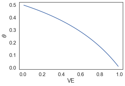
When we have zero vaccine efficacy, \(\theta\) is 0.5, which means that the number of cases in the vaccinated group is no better than that in the placebo group (in fact they are the same number of cases).

Posterior calculations

In the Bayesian framework, we want to know the posterior \(p(\text{VE}>0.3 \vert x)\), where \(x\) is the observed data (i.e. \(c_v\) and \(c_p\)). However, in reality we are not directly modeling VE. Instead, as per our definitions above, we are going to model based on the case rate \(\theta\). This is in part because \(\theta\) is a proportion and ranges from 0 to 1, hence we can easily place a prior based on the beta distribution, which is also bounded to (0,1). From our definitions above, we can easily see by knowing \(\theta\), we also know \(\text{VE}\), and vice versa. Therefore, the posterior \(p(\text{VE}>0.3 \vert x)\) is equivalent to \(p(\theta < \frac{1-0.3}{2-0.3}) \vert x)\), or \(p(\theta<0.4117647 \vert x)\), assuming a 1:1 design with equal surveillance times.

Remember, by Bayes’ rule,

\[\begin{align*} p(\theta \vert x) &\propto p(x \vert \theta) p(\theta) \\ \text{posterior} &\propto \text{likelihood} \times \text{prior} \end{align*}\]

The data \(x\) follows a binomial distribution, as we are asking the number of cases in the vaccinated group out of a total \(n\) cases, with the probability of such cases being in the vaccinated group as \(\theta\). We can define our prior for \(\theta\) as following a beta distribution. Hence,

\[\begin{align*} x &\sim \text{Bin}(n, \theta) \\ \theta &\sim \text{Beta}(\alpha, \beta) \\ \end{align*}\]

We can expand the expressions for our posterior, based on the likelihood and prior distributions,

\[\begin{align*} p(\theta \vert x) &\propto p(x \vert \theta) p(\theta) \\ &\propto \text{Bin}(c_v; n, \theta) \times \text{Beta}(\theta; \alpha, \beta) \\ &\propto {n \choose c_v } \theta^{c_v} (1-\theta)^{c_p} \frac{\Gamma(\alpha+\beta)}{\Gamma(\alpha)\Gamma(\beta)} \theta^{\alpha-1} (1-\theta)^{\beta-1} \\ &\propto \theta^{c_v} (1-\theta)^{c_p} \theta^{\alpha-1} (1-\theta)^{\beta-1} \\ &\propto \theta^{\alpha+c_v-1} (1-\theta)^{\beta+c_p-1} \\ \end{align*}\]

But the last expression is just another beta distribution, so the posterior can be expressed as,

\[\theta \vert x \sim \text{Beta}(\alpha + c_v, \beta + c_p)\]

This is also why beta is a conjugate prior for the binomial distribution, since the posterior is also a beta distribution. We won’t go into more details here, but the posterior predictive distribution is then a beta-binomial distribution.

What prior can we choose? Well if we are interested in testing the posterior \(p(\theta<0.4117647 \vert x)\), we can set the prior beta distribution such that the mean is this value. That is indeed what Pfizer/BioNTech have done - the prior used was Beta(0.700102, 1), so the mean is 0.700102/(0.700102+1) ≈ 0.4118.

Now to calculate the posterior \(p(\theta<0.4117647 \vert x)\), this is simply the CDF of the posterior beta distribution up to 0.4117647. In actual clinical trial results (as opposed to the clinical design), there may be slight differences in surveillance times between vaccinated and placebo groups and this can be account for. Namely, \(p(\text{VE} > 0.3 \vert x)\) is equivalent to \(p(\theta < \frac{r(1-0.3)}{1+r(1-0.3)} \vert x)\).

The 95% credible interval can be obtained via calculating the posterior probabilities at the 2.5th and 97.5th percentile. The lower/upper bound \(\theta\) can then be used to derive the upper/lower bound VE values (with surveillance time adjustment using \(r\)).

Before moving to the next section, we will just explore the effects of different \(\theta\) values on the likelihood and posterior, using the prior we’ve discussed. As an example, we will set 150 total cases, and vary the number of observed cases in the vaccinated group.

import numpy as np
import scipy.stats as st
import matplotlib.pyplot as plt

c_vs = np.array([10, 25, 50, 75]) # no. cases in vaccinated group
c_ps = 150 - c_vs # no. cases in placebo group
a = 0.700102 # param a in prior
b = 1 # param b in prior

fig,ax = plt.subplots(1,3, figsize=(15,5))
plt.subplots_adjust(wspace=0.3)
t = np.linspace(0, 0.7, 200) # theta values

prior_plotted = False
for c_v, c_p in zip(c_vs, c_ps):
    a_p = a + c_v # param a in posterior
    b_p = b + c_p # param b in posterior

    # prior
    if not prior_plotted:
        y_prior = st.beta.pdf(t, a, b)
        ax[1].plot(t, y_prior, c='k')
        ax[1].set(title=f'Prior ~ Beta({a},{b})', xlabel=r'$\theta$', ylabel=r'p($\theta$)')
        prior_plotted = True # just need to plot prior once

    # likelihood
    y_lik = st.binom.pmf(c_v, c_v+c_p, t)
    ax[0].plot(t, y_lik)
    ax[0].set(title='Likelihood', xlabel=r'$\theta$', ylabel=r'p(x|$\theta$)')

    # posterior
    y = st.beta.pdf(t, a_p, b_p)
    ax[2].plot(t, y)
    ax[2].set(title='Posterior', xlabel=r'$\theta$', ylabel=r'p($\theta$|x)')

We see the following,

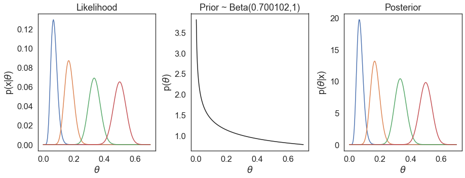
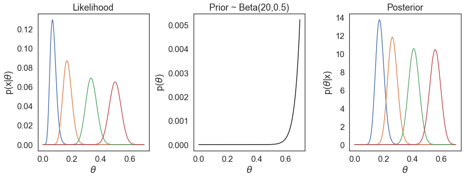
We do not observe the prior having a large influence in our estimations of \(\theta\). On the other hand, if we choose another vastly different prior, e.g. Beta(20, 0.5), we see our posterior estimations are much more influenced by the prior.

In fact the chosen prior Beta(0.700102,1) is what Pfizer/BioNTech referred to as a minimally informative prior - since it has no large influence in our estimations. This prior is defined really just so that the mean corresponds to VE=0.3 - a low expectation of VE, while the uncertainty for \(\theta\) in the prior remains very large. If we examine the 95% credible interval of Beta(0.700102,1), this range is (0.0052, 0.9645) for \(\theta\), corresponding to a 95% credible interval for VE of (-26.16, 0.9948) - this covers essentially the entire range of VE in our prior belief.

Success boundaries

Once we have calculated P(VE>0.3|data), we still need to know at what threshold do we consider our results a success. If the probability of VE > 30% is only 50%, clearly we are not confident in our claim of vaccine efficacy.

Because there are interim analyses performed, we need to account for this in order to keep the overall type I error at a pre-defined level (e.g. 2.5%). Technically this is a frequentist concept, as we have a null hypothesis and corresponding test statistic, in which we reject at a pre-defined alpha level. With interim studies, traditionally in the frequentist approach, we use alpha spending functions (e.g. Lan-DeMets O’Brien-Fleming) that describes how much alpha we ‘spend’ at each interim analysis so the overall alpha is kept (‘protected’) at e.g. 2.5%. In practice, this then defines the alpha to accept/reject the null hypothesis at any given interim analysis. With the Bayesian trial design, this frequentist characteristic can be incorporated via determining thresholds for the posterior probabilities (i.e. P(VE>0.3|data)), such that the overall type I error is controlled at a desired level - hence somewhat of a hybrid frequentist/Bayesian strategy.

In the Pfizer/BioNTech study, the success boundaries were defined as P(VE>0.3|data) > 0.995 and >0.986 for interim and primary analyses, respectively. The boundaries can be derived based on simulations and/or sensitivity analyses (it was unclear the exact methods used in the Pfizer/BioNTech study). From a given boundary, we can also derive the design operating characteristics. This would be a post in of itself and we will not delve deeper here.

COVID-19 VE calculations

The reported COVID-19 efficacy results are as follows,

	Vaccinated group		Placebo group
Developer [ref]	no. cases / total no.	surveillance time⁶	no. cases / total no.	surveillance time⁶
Pfizer/BioNTech⁷	8/18,198	2.214	162/18,325	2.222
Moderna⁸	11/14,134	3.274	185/14,073	3.333
AstraZeneca/Oxford⁹	30/5807	0.680	101/5829	0.677

While only the Pfizer/BioNTech trial used Bayesian analyses. Our goal here is to apply the same Bayesian methodology on all three trial results. We can calculate the VE as 1-IRR, and the 95% credible interval and P(VE>30%|data) calculated using the beta-binomial model with Beta(0.700102, 1) as the prior and with adjustment for surveillance time.

import scipy.stats as st

def calc_theta(VE, r=1):
    # calculate case rate (theta) given VE and surveillance time ratio
    return r*(1-VE) / (1+r*(1-VE))

def calc_VE(theta, r=1):
    # calculate VE given case rate (theta) and surveillance time ratio
    return 1 + theta/(r*(theta-1))

def VE_95ci_betabinom(c_v, c_p, t_v, t_p):
    '''
    Calculates vaccine efficacy (VE) and 95% credible interval
    based on beta-binomial model
    
    params:
        c_v: number of cases in vaccinated group
        c_p: number of cases in placebo group
        t_v: surveillance time in vaccinated group
        t_p: surveillance time in placebo group
    '''
    
    a = 0.700102 + c_v
    b = 1 + c_p
    irr_v = c_v/t_v
    irr_p = c_p/t_p
    r = t_v/t_p
    
    # VE
    VE = 1 - irr_v/irr_p
    
    # confidence interval
    theta_ci_lower = st.beta.ppf(0.025, a, b)
    theta_ci_higher = st.beta.ppf(0.975, a, b)
    VE_ci_lower = calc_VE(theta_ci_higher, r)
    VE_ci_upper = calc_VE(theta_ci_lower, r)
    
    # P(VE>30%|data)
    p_ve30plus = st.beta.cdf(calc_theta(0.3, r), a, b)

    print(f'VE: {VE*100:.2f} ({VE_ci_lower*100:.2f} - {VE_ci_upper*100:.2f}); ' +
          f'P(VE>30%|data): {p_ve30plus:0.30f}')

# calculate VE and 95% CI
VE_95ci_betabinom(8, 162, 2.214, 2.222) # Pfizer/BioNTech
VE_95ci_betabinom(11, 185, 3.274, 3.333) # Moderna
VE_95ci_betabinom(30, 101, 0.680, 0.677) # AstraZeneca/Oxford

Our resulting calculations are as follows,

Developer	VE % (95% Credible Interval)	Posterior P(VE>30%)
Pfizer/BioNTech	95.04 (90.32 - 97.62)	>0.999999
Moderna	93.95 (89.19 - 96.76)	>0.999999
AstraZeneca/Oxford	70.43 (56.00 - 80.48)	>0.999995

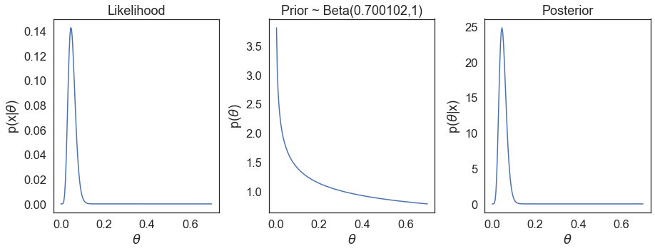
Not surprisingly the calculations for VE and posterior match exactly the results reported in Table 2 in the Pfizer/BioNTech study⁷. Due to us using the Bayesian estimations here, we expectedly observe slight differences in values for the Moderna and AstraZeneca/Oxford studies. We can also see the underlying likelihood, prior, and posterior distributions based on the actual reported cases for the e.g. Pfizer/BioNTech study,

Bayesian distributions for Pfizer/BioNTech COVID-19 study, based on 8 and 162 reported cases in the vaccinated and placebo groups, respectively.

It is important to note there are additional differences amongst the trials, such as criteria for defining confirmed COVID-19 cases, so the comparisons here are only for didactical purposes. Moreover, the emergence of SARS-CoV-2 mutant variants means more recent and/or upcoming clinical trials are run on a background of different viral genetic variants population (such as Johnson & Johnson’s phase 3 trial in South Africa, where B.1.351 mutant is the most prevalent). This further confounds the comparison of vaccine efficacy and effectiveness in the real-world.

Natalie Dean’s twitter posts
Kranz (Nov, 2020) and posts therein
Date (Nov 2020)
Powell (Nov, 2020) and posts therein
Graziani (2020) medrxiv
Halloran et al. 1999 Epidemiol Rev. 21(1), 73-88

References/footnotes

FDA, Development and Licensure of Vaccines to Prevent COVID-19, Guidance for Industry. June 2020. link ↩
Some primary endpoints also include safety, as some clinical trials are combined Phase 1/2/3 trials. The exact criteria for confirmed COVID cases is further described in protocols. The table provided focused only on the measure of efficacy endpoint. ↩ ↩²
As all studies have interim analyses, the success criteria was defined such that the overall type I error was protected at predefined levels (2.5% for BNT162b2 and mRNA-1273; 5% for AZD1222). The success boundary here details only that of the planned primary analysis. Some trials have passed the success boundary in interim studies. ↩
Success boundaries as were planned in study protocol. Actual analyses reported in Baden et al. were based on an interim study where the relevant success threshold for p-value was 0.0049 (stated in FDA Briefing Document on Moderna COVID-19 Vaccine, page 23) - which was based on the O’Brien Fleming boundary at the time of the first interim analysis. The p-value was found to be <0.0001, surpassing the threshold. ↩
The trial is a phase 1/2/3 trial with efficacy as primary endpoints in the pivotal phase 2/3 trial. There were two primary endpoints, one with vaccinated group consisting of participants without evidence of infection prior to vaccination; and other of participants with and without evidence of infection prior to vaccination. We will only focus on the former in this post. ↩
Total time in 1000 person-years. The surveillance time in Pfizer/BioNTech was provided. The surveillance times in Moderna and Astrazeneca studies we have calculated (as cases/incidence rate), given they have provided the incidence rate and the number of cases. ↩ ↩²
Polack et al. 2020 N Eng J Med 383(27), 2603-2615 link ↩ ↩²
Baden et al. 2020 N Eng J Med link ↩
Voysey et al. 2021 Lancet 9;397(10269), 99-111 link ↩

Share on

Twitter Facebook LinkedIn

Boyang Zhao

Vaccine efficacies (with COVID-19 examples) - Bayesian posterior VE/CI calculations

Vaccine efficacy

Select COVID-19 vaccines