
Expectation-maximization in general and for Gaussian mixtures
In statistical inference, we want to find what is the best model parameters given the observed data. In the frequentist view, this is about maximizing the likelihood (MLE). In Bayesian inference, this is in maximizing the posterior. When we maximize the likelihood (often log-likelihood, as this is easier to optimize because of its benefits of monotonic transformation and numerical stability), we are asking,
\[\arg \max_{\theta} \ln p(x; \theta)\]However, what if there are latent variables? Meaning if the model with \(\theta\) parameters generating hidden variables \(z\) and observed data \(x\)? We need to solve the MLE of the form,
\[\arg \max_{\theta} \ln p(x; \theta) = \arg \max_{\theta} \ln \int p(x, z; \theta) \,dz\]where we now need to marginalize out the \(z\), so we are maximizing the marginal log-likelihood. Let us see why this is difficult with an example.
Motivation
Consider the following Gaussian mixture, consisting of \(K\) Gaussian distributions,
\[p(x)=\sum_{k=1}^{K}\pi_k \mathcal{N}(x; \mu_k, \sigma^2_k)\]where \(\pi\) is a mixing coefficient that attributes the proportion of each component Gaussian. The \(\pi\) has the property that the sum add up to 1, i.e. \(\sum \pi_k = 1\). This ensures \(p(x)\) is a probability density function.
The likelihood function and the log-likelihood are,
\[\mathcal{L}(\theta) = \prod_i p(x_i; \theta) = \prod_i \sum_k \pi_k \mathcal{N}(x_i; \mu_k, \sigma^2_k)\] \[\ell(\theta) = \sum_i \ln p(x_i; \theta) = \sum_i \ln \sum_k \pi_k \mathcal{N}(x_i; \mu_k, \sigma^2_k)\]where \(\theta \in \{\pi_k, \mu_k, \sigma^2_k\}, k \in \{1..K\}\)
We can try to maximize the log-likelihoods by taking the derivatives. Let’s try this for one of the model parameters, \(\mu_k\). We will use \(\phi_k(x_i) = \mathcal{N}(x_i; \mu_k, \sigma^2_k)\) to simplify the notations below,
\[\begin{align*} \frac{\partial \ell(\theta)}{\partial \mu_k} &= \sum_i \frac{1}{\sum_k \pi_k \phi_k(x_i)} \pi_k \frac{\partial \phi_k(x_i)}{\partial \mu_k} \\ &= \sum_i \frac{\pi_k \phi_k(x_i)}{\sum_k \pi_k \phi_k(x_i)} \frac{1}{\phi_k(x_i)} \frac{\partial \phi_k(x_i)}{\partial \mu_k} \\ &= \sum_i \frac{\pi_k \phi_k(x_i)}{\sum_k \pi_k \phi_k(x_i)} \frac{\partial \ln \phi_k(x_i)}{\partial \mu_k} \\ \end{align*}\]We see there is an issue. The expression \(\frac{\partial \ln \phi_k(x_i)}{\partial \mu_k}\) is familiar and is just the derivative of the log-likelihood for a single Gaussian - which we can use to estimate its model parameters. However, now there is a weight term \(\frac{\pi_k \phi_k(x_i)}{\sum_k \pi_k \phi_k(x_i)}\) in front, so it is as if we are maximizing a weighted log-likelihood. Unfortunately this weight term depends on the model parameters we are also trying to estimate - hence lies the issue.
We will reformulate the Gaussian mixture in a different way and intuitively see how we can potentially estimate the model parameters. We will create a latent variable \(z \in \{1 .. K\}\) indicating that a given data point came from the kth Gaussian. We define,
\[p(z{=}k) = \pi_k\]With this, the conditional, joint, and marginal distributions are,
\[p(x \vert z{=}k) = \mathcal{N}(x; \mu_k, \sigma^2_k)\] \[p(x,z{=}k) = p(z{=}k) p(x \vert z{=}k) = \pi_k \mathcal{N}(x; \mu_k, \sigma^2_k)\] \[p(x) = \sum_{k=1}^{K} p(x,z{=}k) = \sum_{k=1}^{K} \pi_k \mathcal{N}(x; \mu_k, \sigma^2_k)\]This decomposes the Gaussian mixture into the latent variable \(z\) and the model parameters \(\theta\). This seems to have complicated the model further. But now, with this formulation, we see that if we know one of these variables, we can derive the other.
Knowing \(\theta\): If we know exactly the model parameters \(\theta\), we can figure out which Gaussian each data point came from. The probability the data point came from the kth Gaussian is,
\[p(z{=}k \vert x;\theta) = \frac{p(x,z{=}k;\theta)}{\sum_k p(x,z{=}k;\theta)}\]In fact this is the weight term in our derivatives earlier and is our posterior probability of \(z\).
Knowing z: If we know \(z\), i.e. which Gaussian the data came from, we no longer need to sum over all the K Gaussian (\(\Sigma_z p(x,z)\)) to maximize our marginal likelihood. Instead, we focus on each subset of \(x\) coming from the kth Gaussian, and can estimate \(\theta_k\) with MLE,
\[\arg \max_{\theta_k} \Sigma_i \ln p(x_i; \theta_k), \forall_i(z_i{=}k)\]However, from this we see the catch-22, viz. if we know which Gaussian the data point came from (the hidden variable \(z\)), then we can maximize our log likelihood and get the estimates of our model parameters; if we know the model parameters, we can calculate the posterior probability of \(z\) to estimate which Gaussian each data point came from.
This in fact is the intuition behind EM, which we will formalize in the next section. Instead of deriving the optimal hidden variable \(z\) and model parameter \(\theta\) at the same time, we will take turns optimizing each until we converge.
Python example
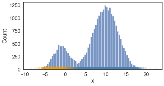
As an example, let us generate the following two-component Gaussian mixture,
import scipy.stats as st
import numpy as np

mu1 = -1
mu2 = 10
sd1 = 2
sd2 = 3
pi_1 = 0.2

k = st.bernoulli(pi_1).rvs(30000)
x1 = st.norm(mu1, sd1).rvs(sum(k==1))
x2 = st.norm(mu2, sd2).rvs(sum(k==0))
x = np.concatenate([x1,x2])
Visually, this looks like
import matplotlib.pyplot as plt
import seaborn as sns

fig = plt.figure(figsize=(8,4))
sns.histplot(x=x)
plt.vlines(x1, 0, 50, color='orange', alpha=0.1);
plt.vlines(x2, 0, 50, color='steelblue', alpha=0.1);
plt.xlabel('x');
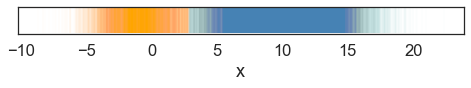
With known \(\theta\), we see the resulting predicted labels (color-coded) match to what we expected,
# with known model params, we can estimate z, i.e. which Gaussian did the data come from
norm_factor = pi_1*st.norm(mu1,sd1).pdf(x) + (1-pi_1)*st.norm(mu2,sd2).pdf(x)
pz_1 = pi_1*st.norm(mu1,sd1).pdf(x) / (norm_factor)
pz_2 = (1-pi_1)*st.norm(mu2,sd2).pdf(x) / (norm_factor)

fig = plt.figure(figsize=(8,0.5))
plt.vlines(x[pz_1>0.5], 0, 0.01, color='orange', alpha=0.01);
plt.vlines(x[pz_2>0.5], 0, 0.01, color='steelblue', alpha=0.01);
plt.yticks([]);
plt.xlabel('x');
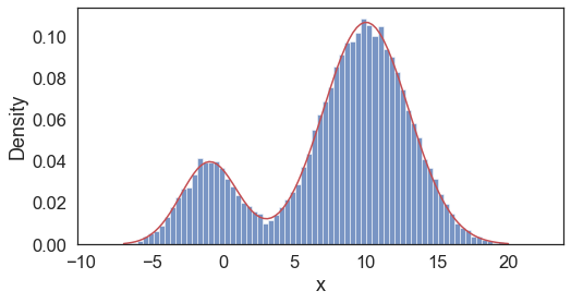
With known \(z\), we can reconstitute the probability density function,
# with known labels, we can estimate the model params
mu1_mle = np.sum(x1)/len(x1)
mu2_mle = np.sum(x2)/len(x2)
sd1_mle = np.std(x1, ddof=0)
sd2_mle = np.std(x2, ddof=0)
pi_est = len(x1)/(len(x1)+len(x2))

print(f'mu_1: {mu1_mle:.2f}; sd_1: {sd1_mle:.2f}; mu_2: {mu2_mle:.2f}; sd_2: {sd2_mle:.2f}; pi: {pi_est:.2f}; ')

t = np.linspace(-7,20,100)
x_est = pi_est*st.norm(mu1_mle, sd1_mle).pdf(t)+(1-pi_est)*st.norm(mu2_mle, sd2_mle).pdf(t)

fig = plt.figure(figsize=(8,4))
plt.plot(t,x_est, color='r')
sns.histplot(x=x, stat='density');
plt.xlabel('x');
Model parameters MLE estimates:
mu_1: -0.98; sd_1: 1.99; mu_2: 10.03; sd_2: 3.00; pi: 0.20;
EM algorithm
Our goal is to maximize the log marginal likelihood for models with latent variables. Because this expression results in an integral (or sum if discrete) inside the log transform, we introduce an arbitrary distribution \(q\) over \(z\) and apply Jensen’s inequality to construct a lower bound on the likelihood,
\[\begin{align*} \sum_i \ln p(x_i;\theta) &= \sum_i \ln \int p(x_i,z_i;\theta) \,dz \\ &= \sum_i \ln \int q(z_i) \frac{p(x_i,z_i;\theta)}{q(z_i)} \,dz \\ &\ge \sum_i \int q(z_i) \ln \frac{p(x_i,z_i;\theta)}{q(z_i)} \,dz \\ &= F(q, \theta) \\ \end{align*}\]The term \(F(q, \theta)\) consists of,
\[\begin{align*} F(q, \theta) &= \sum_i \int q(z_i) \ln p(x_i,z_i;\theta) \,dz - \sum_i \int q(z_i) \ln q(z_i) \,dz \\ &= \sum_i \text{E}_{z_i \sim q}[\ln p(x_i,z_i;\theta)] + \sum_i H(q) \\ \end{align*}\]The expression \(F(q, \theta)\) is a lower bound of our marginal likelihood and depends on our choice of the distribution \(q\) and our estimates of \(\theta\). To have the tightest bound at our current estimate of \(\theta\), we want to maximize \(F(q, \theta^{(t)})\) with respect to \(q\), to derive a distribution \(q^{(t+1)}\). It can be shown that the tightest bound at our current \(\theta\) estimate is when we hold the above inequality with equality, resulting in the optimal \(q\) being the posterior distribution of \(z\) given \(x\) and \(\theta^{(t)}\). With this bound, we can maximize \(F(q^{(t+1)}, \theta)\) with respect to \(\theta\) to get a better estimate of \(\theta\), which is also a better estimate for our marginal likelihood. This effectively is the expectation and maximization steps in the EM algorithm.
Before formalizing each step, we will introduce the following notation,
\[Q(\theta; \theta^{(t)}) = \sum_i \text{E}_{z_i \vert x_i; \theta^{(t)}}[\ln p(x_i,z_i;\theta)]\]where \(Q(\theta; \theta^{(t)})\) is the lower bound of the marginal likelihood at a given \(\theta^{(t)}\) with respect to the posterior distribution of z given \(x\) and \(\theta^{(t)}\). This expression can be thought of as the expected complete log-likelihood. Since \(H(q)\) does not depend on \(\theta\), maximizing \(F(q, \theta)\) with respect \(\theta\) is equivalent to maximizing the complete log-likelihood.
Expectation step: Maximize \(F(q, \theta)\) with respect to \(q\). The solution (i.e. the tightest bound) at our current estimate of \(\theta\) is the posterior distribution of \(z\) given \(x\) and \(\theta^{(t)}\). Thus, in practice, we need to calculate,
\[\begin{align*} q^{(t+1)} &= \mathop{\operatorname{arg\,max}}_{q} F(q, \theta^{(t)}) \\ &=p(z \vert x; \theta^{(t)}) \end{align*}\]Maximization step: Maximize \(F(q, \theta)\) with respect to \(\theta\). In other words, maximize the expected complete log-likelihood,
\[\begin{align*} \theta^{(t+1)} &= \mathop{\operatorname{arg\,max}}_{\theta} F(q^{(t+1)}, \theta) \\ &= \mathop{\operatorname{arg\,max}}_{\theta} Q(\theta; \theta^{(t)}) \\ &= \mathop{\operatorname{arg\,max}}_{\theta} \sum_i \text{E}_{z_i \vert x_i; \theta^{(t)}} [\ln p(x_i,z_i ; \theta)] \end{align*}\]Gaussian mixture with EM
Back to our example of the Gaussian mixture model, based on our discussion of EM above, we see that,
Expectation step: We calculate \(\gamma=q(z)\), the probability of the data point \(x\) belonging to each of the component Gaussian distributions. \(\gamma\) is also known as the responsibility, i.e. how much each kth Gaussian is responsible for the data.
The probability that the data point \(x_i\) came from the kth Gaussian is,
\[\gamma_{ik} = q(z_i{=}k) = p(z_i{=}k \vert x_i;\theta) = \frac{p(x_i,z_i{=}k;\theta)}{\sum_k p(x_i,z_i{=}k;\theta)} = \frac{ \pi_k \mathcal{N}(x_i;\mu_k, \sigma^2_k) }{\sum_k \pi_k \mathcal{N}(x_i;\mu_k, \sigma^2_k)}\]Maximization step: We maximize the complete log-likelihood
\[\begin{align*} Q(\theta; \theta^{(t)}) &= \sum_i \text{E}_{z_i \vert x_i; \theta^{(t)}} [\ln p(x_i,z_i; \theta)] \\ &= \sum_i \sum_k \gamma_k \ln \left( \pi_k \mathcal{N}(x_i; \mu_k, \sigma^2_k) \right) \end{align*}\]To maximize this expression with respect to each of the parameters, we take the derivatives,
\[\begin{align*} \frac{\partial Q(\theta; \theta^{(t)})}{\partial \mu_k} &= 0 \\ \frac{\partial Q(\theta; \theta^{(t)})}{\partial \sigma^2_k} &= 0 \\ \frac{\partial Q(\theta; \theta^{(t)})}{\partial \pi_k} &= 0 \end{align*}\]The solution is,
\[\begin{align*} \mu_k^{(t+1)} &= \frac{\Sigma_{i=1}^n \gamma_{ik}^{(t)} x_i}{\Sigma_{i=1}^n \gamma_{ik}^{(t)}} \\ {\sigma^2}_k^{(t+1)} &= \frac{\Sigma_{i=1}^n \gamma_{ik}^{(t)} (x_i-\mu_k^{(t+1)})^2}{\Sigma_{i=1}^n \gamma_{ik}^{(t)}} \\ \pi_k^{(t+1)} &= \frac{\Sigma_{i=1}^n \gamma_{ik}^{(t)}}{n} \\ \end{align*}\]with \(n\) denoting the total number of observed data points.
Python example
Using the example earlier, our Python implementation is as follows,
def EM_Gaussian(mu_init, sd_init, pi_init, n_iter=1000):
    # EM for Gaussian mixture models
    mu = mu_init
    sd = sd_init
    pi = pi_init
    K = len(pi_init) # number of Gaussians

    for n in range(n_iter):
        # Expectation step
        # calculate responsibilities for each Guassian
        norm_factor = 0
        for mu_k, sd_k, pi_k in zip(mu, sd, pi):
            norm_factor += pi_k*st.norm(mu_k,sd_k).pdf(x)

        pz = [[],[]]
        for k in range(K):
            pz[k] = pi[k]*st.norm(mu[k],sd[k]).pdf(x) / (norm_factor)

        # Maximization step
        # calculate the model params for next step
        for k in range(K):
            mu[k] = np.sum(pz[k]*x) / np.sum(pz[k])
            sd[k] = (np.sum(pz[k]*(x-mu[k])**2) / np.sum(pz[k]))**0.5
            pi[k] = np.sum(pz[k])/len(pz[k])

    return mu, sd, pi

# run EM
mu_est, sd_est, pi_est = EM_Gaussian([0, 0], [1, 1], [0.4, 0.5], n_iter=1000)

# print out estimated params
for mu_k, sd_k, pi_k, k in zip(mu_est, sd_est, pi_est, np.arange(len(pi_est))+1):
    print(f'mu_{k}: {mu_k:.2f}; sd_{k}: {sd_k:.2f}; pi_{k}: {pi_k:.2f};')

# plot results
t = np.linspace(-7,20,100)
x_est = pi_est[0]*st.norm(mu_est[0], sd_est[0]).pdf(t) + pi_est[1]*st.norm(mu_est[1], sd_est[1]).pdf(t)

fig = plt.figure(figsize=(8,4))
plt.plot(t,x_est,color='r')
sns.histplot(x=x, stat='density');
Final estimated model parameters:
mu_1: -0.99; sd_1: 1.99; pi_1: 0.20;
mu_2: 10.01; sd_2: 3.00; pi_2: 0.80;
Above we show snapshots of estimated PDF at select iterations until convergence. Our resulting final approximations match very closely to the original model parameters used to generate this data.
References/resources
There are an endless list of online resources discussing expectation-maximization with varying degrees of clarity. Below are a select few that I found particularly good, and of which this post is loosely based on,
Leave a comment