Gibbs sampling of multivariate probability distributions
This is a continuation of a previous article I have written on Bayesian inference using Markov chain Monte Carlo (MCMC). Here we will extend to multivariate probability distributions, and in particular looking at Gibbs sampling. I refer the reader to the earlier article for more basic introductions to Bayesian inference and MCMC.
Gibbs sampling basics
Monte Carlo methods are essentially about sampling from distributions, and calculating integrals,
\[E_{p(x)}[ g(x) ] = \int g(x)p(x) \,dx \approx \frac{1}{N} \sum_{t=1}^N g(x^{(t)})\]In this above equation, we want to approximate the expected value of \(g(x)\) with random variable \(X\) that is of distribution \(p(x)\).
MCMC is designed when we cannot directly sample from \(p(x)\). Instead we sample from a distribution proportional to it, with the resulting stationary distribution of the Markov chain equaling to \(p(x)\). When the \(p(\boldsymbol{x})\) is multivariate, in the standard Metropolis-Hastings algorithm, we would draw from a proposal distribution that is a joint distribution (to propose simultaneously the new values for \(x_1\), \(x_2\), etc). In Gibbs sampling, we instead alternatively sample from full conditional distributions, e.g. \(p(x_1 \vert \boldsymbol{x_{-1}})\). The end result is the same - we have an approximation of the joint distribution \(p(\boldsymbol{x})\).
Steps
- Set initial value for \(\boldsymbol{x} = (x_1, x_2, … x_k)\)
-
For \(t\) = 1, 2, 3, … \(N\)
a. Propose new \(x_i^*\) based on \(p(x_i^* | \boldsymbol{x}_{-i}^{(t)})\) where \(\boldsymbol{x}_{-i}^{(t)}\) is the set of all variables in \(\boldsymbol{x}^{(t)}\) except \(x_i\)
b. Repeat for the other random variables in \(\boldsymbol{x}^{(t)}\)
c. Set \(\boldsymbol{x}^{(t+1)} = (x_1^*, x_2^* … x_k^*)\)
After burn-in, the series of \((x_1,x_2 … x_k)\) constitute the approximation of the joint distribution.
Thus, with Gibbs sampling, we just need to know the full conditional distributions in approximating the joint distribution. This is useful in cases where the joint distribution cannot be sampled directly, but the sampling from full conditional distributions is readily accessible. From the joint distribution, we can also derive approximation of marginal distributions (e.g. \(p(x_1)\)) by examining subset of the variables, or expected values (e.g. \(E[ x_1 ]\)).
Gibbs sampling as special case of Metropolis-Hastings
In fact, Gibbs sampling is a special case of the Metropolis-Hastings algorithm. Given the acceptance ratio in MH,
\[r(x^*, x^{(t)}) = \frac{f(x^*)q(x^{(t)}|x^*)}{f(x^{(t)})q(x^*|x^{(t)})}\]with Gibbs sampling, our \(f(x)\) is a probability distribution \(p(\boldsymbol{x})\) and our proposal distribution is the full conditional distributions of \(p(\boldsymbol{x})\). At each proposal step, the acceptance ratio is essentially,
\[\begin{align*} r(x_i^*, x_i^{(t)} ) &= \frac{ p(x_i^*,x_{-i}^{(t)} ) p(x_i^{(t)}|x_{-i}^{(t)})} {p(x_i^{(t)}, x_{-i}^{(t)} ) p(x_i^* |x_{-i}^{(t)})} \\ &= \frac{p(x_i^* | x_{-i}^{(t)})p(x_{-i}^{(t)}) p(x_i^{(t)} | x_{-i}^{(t)})} {p(x_i^{(t)}|x_{-i}^{(t)}) p(x_{-i}^{(t)}) p(x_i^*|x_{-i}^{(t)})} \\ &= 1 \end{align*}\]Hence with Gibbs sampling, it is a MH algorithm with acceptance ratio always equaling to 1.
Example | Multivariate Gaussian distributions
As an example, we will examine multivariate Gaussian distributions, \(\boldsymbol{X}{\sim}\mathcal{N}(\boldsymbol{\mu,\Sigma})\). The conditional Gaussian distribution can be derived analytically as,
\[(\boldsymbol{x_1 | x_2=a}) \sim \mathcal{N} ( \boldsymbol{\bar{\mu}}, \boldsymbol{\bar{\Sigma}} )\]where,
\[\boldsymbol{ \bar{\mu} } = \boldsymbol{ \mu_1 + \Sigma_{12} \Sigma_{22}^{-1} (a - \mu_2) }\] \[\boldsymbol{ \bar{\Sigma} } = \boldsymbol{ \Sigma_{11} - \Sigma_{12} \Sigma_{22}^{-1} \Sigma_{21} }\]with the partitions,
\[\boldsymbol{\mu} = \begin{bmatrix} \boldsymbol{\mu_1 \\ \mu_2} \end{bmatrix}\] \[\boldsymbol{\Sigma} = \begin{bmatrix} \boldsymbol{ \Sigma_{11} } & \boldsymbol{ \Sigma_{12} } \\ \boldsymbol{ \Sigma_{21} } & \boldsymbol{ \Sigma_{22} } \end{bmatrix}\]For Gibbs sampling, the \(1\) is the \(i\)th variable to be sampled, and \(2\) are the \(-i\) indices (the set of all variables except \(x_i\)). In the example below, we will use a bivariate Gaussian with the following parameters,
\[\boldsymbol{\mu} = \begin{bmatrix} -2 \\ 1 \end{bmatrix}\] \[\boldsymbol{\sigma} = \begin{bmatrix} 1 & 0.8 \\ 0.8 & 1 \end{bmatrix}\]We first define our parameter values,
import numpy as np
import scipy.stats as st

np.random.seed(10)

mu = np.array([-2, 1])
sigma = np.array([[1, 0.8], [0.8, 1]])
cov = np.power(sigma, 2)
Then we will perform the Gibbs sampling steps, with an initial x = [0, 0]. Again our goal here is to approximate this joint bivariate distribution via sampling of its conditional distributions.
class guassian_prob:
    # class for sampling from conditional Gaussian distribution

    def __init__(self, mu: np.ndarray, cov: np.ndarray):
        # initialize with mean and covariance matrix

        # take care of some typing
        mu = np.array(mu) if type(mu) is list else mu
        cov = np.array(cov) if type(cov) is list else cov

        self.mu = mu
        self.cov = cov

    def sample_conditional(self, x: np.ndarray, idx: list):
        # sampling from a conditional distribution
        # given X, and draw from p(X_idx | X_rest), where idx is index in array X

        # take care of some typing
        idx = [idx] if type(idx) is int else idx
        x = [x] if type(x) is int else x
        x = np.array(x) if type(x) is list else x

        # get the indices of variables to be conditioned on
        idx_not = [i for i in list(range(len(self.mu))) if i not in idx]

        # get the matrix components
        mu1 = self.mu[idx]
        mu2 = self.mu[idx_not]
        cov11 = self.cov[np.ix_(idx, idx)]
        cov22 = self.cov[np.ix_(idx_not, idx_not)]
        cov12 = self.cov[np.ix_(idx, idx_not)]
        cov21 = self.cov[np.ix_(idx_not, idx)]
        a = x[idx_not]

        # calculate conditional matrices
        mu_cond = mu1 + np.matmul(np.matmul(cov12, np.linalg.inv(cov22)), (a - mu2))
        cov_cond = cov11 - np.matmul(np.matmul(cov12, np.linalg.inv(cov22)), cov21)

        x_new = st.multivariate_normal(mu_cond, cov_cond).rvs()

        return x_new

    def sample(self, n):
        # direct sampling of the joint distribution
        return st.multivariate_normal(mean=mu, cov=cov).rvs(n)


def mcmc_gibbs(prob_func, x_init, n_iter=1000):
    # Gibbs sampling, given a conditional distribution function (class)

    xs = []
    x_sample = x_init # initial x values

    for i in range(n_iter):
        for j in range(len(x_sample)):
            x_sample[j] = prob_func.sample_conditional(x_sample, j)

        xs.append(x_sample.copy())

    return np.vstack(xs)

prob = guassian_prob(mu, cov)
xs = mcmc_gibbs(prob, [0,0], n_iter=5000)
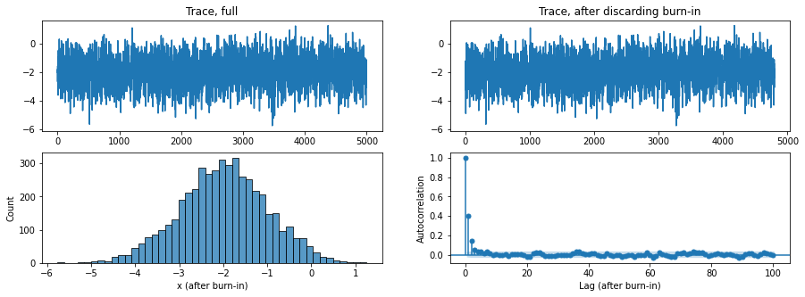
From our trace and auto-correlations of the results, we see that we have fairly independent sampling with a very small burn-in. We chose to discard the first 200 samples.

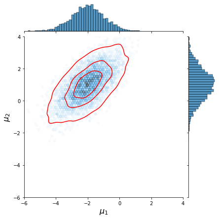
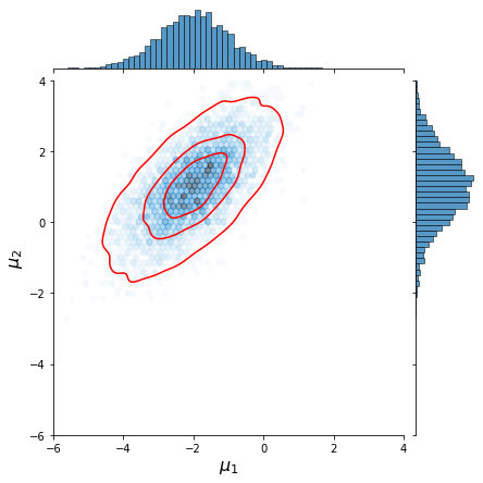
Now let us plot the resulting joint distributions,
import seaborn as sns

# joint distribution based on Gibbs sampling
g = sns.jointplot(x=xs[:,0], y=xs[:,1], xlim=[-6,4], ylim=[-6,4], alpha=0.5, kind='hex');
g.plot_joint(sns.kdeplot, color="r", zorder=1, levels=4);
g.set_axis_labels('$\mu_1$', '$\mu_2$', fontsize=16);

# joint distribution based on direct sampling
xs_direct = st.multivariate_normal(mean=mu, cov=cov).rvs(size=4800)
g = sns.jointplot(x=xs_direct[:,0], y=xs_direct[:,1], xlim=[-6,4], ylim=[-6,4], alpha=0.5, kind='hex');
g.plot_joint(sns.kdeplot, color="r", zorder=1, levels=4);
g.set_axis_labels('$\mu_1$', '$\mu_2$', fontsize=16);
We observe that the approximation by Gibbs sampling closely resembles that performed via direct sampling.
| Gibbs sampling | Direct sampling of joint distr. |
|---|---|
 |
 |
Gibbs sampling for Bayesian inference
Remember that in Bayesian inference, we are interested in inferring the posterior distribution of model parameters. By Bayes’ rule, we have,
\[p(\theta|x) \propto p(x|\theta)p(\theta)\]In standard Metropolis-Hastings algorithm, we sample from a joint proposal distribution (for multivariate cases) and multiply by the unnormalized posterior (\(p(x \vert \theta)p(\theta)\)) in deciding whether to accept or reject the proposed parameter values in each step. With Gibbs sampling, we are effectively sampling from the full conditional posterior distributions, \(p(\theta_i \vert \theta_{-i}, x)\), and always accept the proposed values. The procedures are the same as discussed earlier.

Leave a comment