
Monte Carlo integration in Python over univariate and multivariate functions
Monte Carlo integration is a basic Monte Carlo method for numerically estimating the integration of a function \(f(x)\). We will discuss here the theory along with examples in Python.
Theory
Suppose we want to solve the integration of \(f(x)\) over a domain \(D\).
\[I = \int_{\boldsymbol{x} \in D} f(\boldsymbol{x}) \,d\boldsymbol{x}\]In the case of a univariate function (i.e. with one variable), the domain is simply one dimensional and the integration is from \(a\) to \(b\).
We can rearrange some terms and express the above equation as,
\[I = \int_{\boldsymbol{x} \in D} \frac{f(\boldsymbol{x})}{p(\boldsymbol{x})} p(\boldsymbol{x}) \,d\boldsymbol{x} = \int_{\boldsymbol{x} \in D} g(\boldsymbol{x})p(\boldsymbol{x}) \,d\boldsymbol{x} = E[ g(\boldsymbol{x}) ]\]In other words, the integration is equivalent to finding the expected value of \(g(x)\), where we have defined \(g(x)=f(x)/p(x)\) over a domain. We can approximate this by sampling \(x\) from the domain for \(N\) times, which means,
\[E[ g(\boldsymbol{x}) ] \approx \frac{1}{N} \sum_{i=1}^{N} g(\boldsymbol{x}_i) = \frac{1}{N} \sum_{i=1}^{N} \frac{f(\boldsymbol{x}_i)}{p(\boldsymbol{x}_i)}\]If we are sampling from a uniform distribution, and let say the function is univariate, this means the probability of drawing any given \(x\) is simply \(p(x)=1/(b-a)\). If we substitute this into the above approximation expression, we see that,
\[\begin{align*} I &= \int_a^b f(x) \,dx \\ \hat{I} &= (b-a) \frac{1}{N} \sum_{i=1}^{N} f(x_i) \end{align*}\]This is effectively calculating the mean value of \(f(x)\) over the interval \(a\) to \(b\) and multiplying by the length of the interval. In other words, we are finding the area of a rectangle with width = interval width and height = expected value of \(f(x)\).
This also works with any dimensions. In case of a univariate function, the domain is simply a line (i.e. \(b-a\)). For a bivariate function, the domain is the area. Generally,
\[\hat{I} = V \frac{1}{N} \sum_{i=1}^{N} f(\boldsymbol{x}_i)\]This means we can approximate the integration by multiplying the domain volume by the expected value of the function over the domain.
Example | Univariate
As an example, in Python, we can perform the following to approximate the integration of \(f(x)=x^2\) from -2 to 2.
import numpy as np

def func1(x):
    # function f(x)=x^2
    return x**2

def func1_int(a, b):
    # analytical solution to integral of f(x)
    return (1/3)*(b**3-a**3)

def mc_integrate(func, a, b, n = 1000):
    # Monte Carlo integration between x1 and x2 of given function from a to b

    vals = np.random.uniform(a, b, n)
    y = [func(val) for val in vals]

    y_mean = np.sum(y)/n
    integ = (b-a) * y_mean

    return integ

print(f"Monte Carlo solution: {mc_integrate(func1, -2, 2, 500000): .4f}")
print(f"Analytical solution: {func1_int(-2, 2): .4f}")
We get the following results,
Monte Carlo solution: 5.3323
Analytical solution: 5.3333
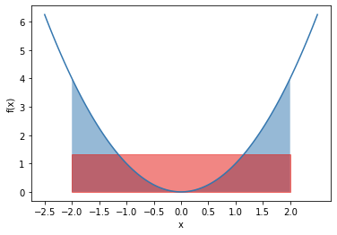
where the Monte Carlo approximation is very close to the analytical solution. Visually, the integration of \(f(x)=x^2\) from -2 to 2 is shown below in blue. The approximation is the rectangle highlighted in red.
Example | Multivariate
We can also perform integration for multivariate functions. The procedure is the same as before. However, instead of sampling over a line (from \(a\) to \(b\)), we now need to sample over a higher-dimensional domain. For simplicity, we will illustrate the integration of a multivariate function over a domain with the same \(a\) and \(b\) for each variable. This means in a function with two variables (x1 and x2), the domain is square shaped; and for function with three variables, cube shaped.
import numpy as np

def func1(x):
    # function f(x)= 10 + sum_i(-x_i^2)
    # for 2D: f(x)= 10 - x1^2 - x2^2
    return 10 + np.sum(-1*np.power(x, 2), axis=1)

def mc_integrate(func, a, b, dim, n = 1000):
    # Monte Carlo integration of given function over domain from a to b (for each parameter)
    # dim: dimensions of function

    x_list = np.random.uniform(a, b, (n, dim))
    y = func(x_list)

    y_mean =  y.sum()/len(y)
    domain = np.power(b-a, dim)

    integ = domain * y_mean

    return integ

# Examples
print("For f(x)= 10 - x1\u00b2 - x2\u00b2, integrated from -2 to 2 (for all x's)")
print(f"Monte Carlo solution for : {mc_integrate(func1, -2, 2, 2, 1000000): .3f}")
print(f"Analytical solution: 117.333")

print("For f(x)= 10 - x1\u00b2 - x2\u00b2 - x3\u00b2, integrated from -2 to 2 (for all x's)")
print(f"Monte Carlo solution: {mc_integrate(func1, -2, 2, 3, 1000000): .3f}")
print(f"Analytical solution: 384.000")
The results
For f(x)= 10 - x12 - x22, integrated from -2 to 2 (for all x’s)
Monte Carlo solution: 117.346
Analytical solution: 117.333
For f(x)= 10 - x12 - x22 - x32, integrated from -2 to 2 (for all x’s)
Monte Carlo solution: 383.888
Analytical solution: 384.000
Example | Multivariate integrated over other domains
The domain over which the integration is performed can be more complicated and difficult to sample from and to calculate its volume. We can for example integrate our bivariate function over a circular domain instead of a square domain. The idea is nonetheless the same — with uniform sampling, we wish to sample over the domain, and approximate the integration via the product of the domain volume and expected value of the function over the domain.
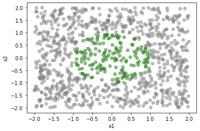
Let’s use the same bivariate function \(f(x)=10-x1^2-x2^2\) and integrate over a unit circle. Uniform sampling over exactly the unit circle is harder than just sampling over a square region (that covers the unit circle). From this we can 1) calculate the area of the domain as the product of the area of the sampled square by the proportion of sampled points inside the domain, 2) the expectation as the mean f(x) of the sampled points inside the domain. Below is a visualization of the sampling (sampled points inside the unit circle shown in green),
In Python, this looks like,
import numpy as np

def func1(x):
    # function f(x)= 10 + sum_i(-x_i^2)
    # for 2D: f(x)= 10 - x1^2 - x2^2
    return 10 + np.sum(-1*np.power(x, 2), axis=1)

def domain_unit_circle(x):
    # integration domain: sum of x^2 <= 1.
    # For 2d, it's a unit circle; for 3d it's a unit sphere, etc
    # returns True for inside domain, False for outside

    return np.power(x,2).sum() <= 1

def mc_integrate(func, func_domain, a, b, dim, n = 1000):
    # Monte Carlo integration of given function over domain specified by func_domain
    # dim: dimensions of function

    # sample x
    x_list = np.random.uniform(a, b, (n, dim))

    # determine whether sampled x is inside or outside of domain and calculate its volume
    inside_domain = [func_domain(x) for x in x_list]
    frac_in_domain = sum(inside_domain)/len(inside_domain)
    domain = np.power(b-a, dim) * frac_in_domain

    # calculate expected value of func inside domain
    y = func(x_list)
    y_mean = y[inside_domain].sum()/len(y[inside_domain])

    # estimated integration
    integ = domain * y_mean

    return integ

print("For f(x)= 10 - x1\u00b2 - x2\u00b2, integrated over unit circle")
print(f"Monte Carlo solution: {mc_integrate(func1, domain_unit_circle, -2, 2, 2, 1000000): .3f}")
print(f"Analytical solution: 29.845")
With results as,
For f(x)= 10 - x12 - x22, integrated over unit circle
Monte Carlo solution: 29.849
Analytical solution: 29.845
As a last example, we can also integrate over multivariate probability distributions. Let’s integrate the following multivariate normal distribution over the unit circle,
\[\boldsymbol{X} \sim \mathcal{N} ( \boldsymbol{\mu}, \boldsymbol{\Sigma} )\]where \(\boldsymbol{\mu} = \begin{bmatrix} 0 \\ 0.5 \\ 1.0 \end{bmatrix}\) and \(\boldsymbol{\Sigma} = \begin{bmatrix} 1 & 0.8 & 0.5 \\ 0.8 & 1 & 0.8 \\ 0.5 & 0.8 & 1 \end{bmatrix}\)
We define these in Python and perform our Monte Carlo integration,
import scipy.stats as st

class func_mvn:
    # multivariate normal given mean and covariance
    def __init__(self, mu, cov):
        self.mu = mu
        self.cov = cov
        self.func = st.multivariate_normal(mu, cov)

    def calc_pdf(self, x):
        return self.func.pdf(x)

mean = np.array([0, 0.5, 1])
cov = np.array([[1, 0.8, 0.5], [0.8, 1, 0.8], [0.5, 0.8, 1]])

f = func_mvn(mean, cov)
fmvn = f.calc_pdf

print("For multivariate normal, integrated over unit circle")
r, x_list, inside_domain = mc_integrate(fmvn, domain_unit_circle, -1, 1, 3, 2000000)
print(f"Monte Carlo solution: {r: .4f}")
print(f"Solution from pmvnEll (shotGroups pkg in R): {0.2018934: .4f}")
As confirmation, we use the pmvnEll function that can integrate multivariate normal distributions over ellipsoids (circles included).
#in R
library(shotGroups)
pmvnEll(r=1, sigma=rbind(c(1,0.8,0.5), c(0.8,1,0.8), c(0.5,0.8,1)), mu=c(0,0.5,1), e=diag(3), x0=c(0,0,0))
With the results closely matching each other,
For multivariate normal, integrated over unit circle
Monte Carlo solution: 0.2020
Solution from pmvnEll (shotGroups pkg in R): 0.2019
Additional comments
Obviously the examples provided are simple and some have analytical solutions and/or Python/R packages for specific cases. But they are useful to get a grasp of the mechanics behind Monte Carlo integration. Clearly the Monte Carlo method described is readily generalizable to more complicated functions with no closed form solutions. In addition, there are many more optimized ways to perform sampling (e.g. stratified sampling, importance sampling, etc) and readers are encouraged to read more into those topics if interested.
Leave a comment