Getting started with Gaussian process regression modeling

Gaussian processing (GP) is quite a useful technique that enables a non-parametric Bayesian approach to modeling. It has wide applicability in areas such as regression, classification, optimization, etc. The goal of this article is to introduce the theoretical aspects of GP and provide a simple example in regression problems.

Multivariate Gaussian distribution

We first need to do a refresher on multivariate Gaussian distribution, which is what GP is based on. A multivariate Gaussian distribution can be fully defined by its mean vector and covariance matrix

\[\boldsymbol{X} \sim \mathcal{N}(\boldsymbol{\mu}, \boldsymbol{\Sigma})\]

There are two important properties of Gaussian distributions that make later GP calculations possible: marginalization and conditioning.

Marginalization

With a joint Gaussian distribution, this can be written as,

\[\begin{bmatrix}\boldsymbol{X} \\ \boldsymbol{Y} \end{bmatrix} \sim \mathcal{N} \bigg( \begin{bmatrix}\boldsymbol{\mu_X} \\ \boldsymbol{\mu_Y} \end{bmatrix}, \begin{bmatrix} \boldsymbol{\Sigma_{XX}} & \boldsymbol{\Sigma_{XY}} \\ \boldsymbol{\Sigma_{YX}} & \boldsymbol{\Sigma_{YY}} \end{bmatrix} \bigg)\]

We can retrieve a subset of the multivariate distribution via marginalization. For example, we can marginalize out the random variable \(Y\), with the resulting \(X\) random variable expressed as follows,

\[p(\boldsymbol{X}) = \int_\boldsymbol{Y} p(\boldsymbol{X}, \boldsymbol{Y}) \,dy = \mathcal{N}(\boldsymbol{\mu_X}, \boldsymbol{\Sigma_{XX}})\]

Note that the marginalized distribution is also a Gaussian distribution.

Conditioning

Another important operation is conditioning, which describes the probability of a random variable given the presence of another random variable. This operation enables Bayesian inference, as we will show later, in deriving the predictions given the observed data.

With conditioning, you can derive for example,

\[p(\boldsymbol{X}|\boldsymbol{Y}) = \mathcal{N}( \boldsymbol{\mu_X} + \boldsymbol{\Sigma_{XY}\Sigma_{YY}^{-1}(Y - \mu_Y)}, \boldsymbol{\Sigma_{XX}} - \boldsymbol{\Sigma_{XY}\Sigma_{YY}^{-1}\Sigma_{YX}} )\]

Like the marginalization, the conditioned distribution is also a Gaussian distribution. This allows the results to be expressed in closed form and is tractable.

Gaussian process

We can draw parallels between a multivariate Gaussian distribution and a Gaussian process. A Gaussian process (GP) is fully defined by its mean function and covariance function (aka kernel),

\[f(\boldsymbol{x}) \sim GP(m(\boldsymbol{x}), k(\boldsymbol{x}, \boldsymbol{x}'))\]

GP can be thought of as an infinite dimensional multivariate Gaussian. This is actually what we mean by GP as being non-parametric — because there are an infinite number of parameters. The mean function, \(m(x)\), describes the mean of any given data point \(x\), and the kernel, \(k(x,x’)\), describes the relationship between any given two data points \(x_1\) and \(x_2\).

As such, GP describes a distribution over possible functions. So when you sample from a GP, you get a single function. In contrast, when you sample from a Gaussian distribution, you get a single data point.

Gaussian process regression

We can bring together the above concepts about marginalization and conditioning and GP to regression. In a traditional regression model, we infer a single function, \(Y=f(\boldsymbol{X})\). In Gaussian process regression (GPR), we place a Gaussian process over \(f(\boldsymbol{X})\). When we don’t have any training data and only define the kernel, we are effectively defining a prior distribution of \(f(\boldsymbol{X})\). We will use the notation \(\boldsymbol{f}\) for \(f(\boldsymbol{X})\) below. Usually we assume a mean of zero, so all together this means,

\[\boldsymbol{f} \sim \mathcal{N}(\boldsymbol{0}, \boldsymbol{K})\]

The kernel \(\boldsymbol{K}\) chosen (e.g. periodic, linear, radial basis function) describes the general shapes of the functions. The same way when you choose a first-order vs second-order equation, you’d expect different function shapes of e.g. a linear function vs a parabolic function.

When we have observed data (e.g. training data, \(\boldsymbol{X}\)) and data points where we want to estimate (e.g. test data, \(\boldsymbol{X}^*\)), we again place a Gaussian prior over \(\boldsymbol{f}\) (for \(f(\boldsymbol{X})\)) and \(\boldsymbol{f^*}\) (for \(f(\boldsymbol{X^*})\)), yielding a joint distribution,

\[\begin{bmatrix}\boldsymbol{f} \\ \boldsymbol{f_*} \end{bmatrix} \sim \mathcal{N}( \boldsymbol{0}, \begin{bmatrix} \boldsymbol{K} & \boldsymbol{K_*} \\ \boldsymbol{K_*^T} & \boldsymbol{K_{*,*}} \end{bmatrix} )\]

The objective here is we want to know what is \(\boldsymbol{f^*}\) for some set of \(x\) values (\(\boldsymbol{X^*}\)) given we have observed data (\(\boldsymbol{X}\) and its corresponding \(\boldsymbol{f}\)). This is effectively conditioning, and in other words it is asking to derive the posterior probability of the function values, \(p(\boldsymbol{f^*|f,X,X^*})\). This is also how we can make predictions — to calculate the posterior conditioned on the observed data and test data points.

Adding noise

The functions described above are noiseless, meaning we have perfect confidence in our observed data points. In the real world, this is not the case and we expect to have some noise in our observations. In the traditional regression models, this can be modeled as,

\[\boldsymbol{Y} = f(\boldsymbol{X}) + \boldsymbol{\epsilon}\]

where \(\boldsymbol{\epsilon} \sim \mathcal{N}(\boldsymbol{0}, \sigma^2 \boldsymbol{I})\). The \(\boldsymbol{\epsilon}\) is the noise term and follows a Gaussian distribution. In GPR, we place the Gaussian prior onto \(f(\boldsymbol{X})\) just like before, so \(f(\boldsymbol{X}) \sim GP(\boldsymbol{0,K})\) and \(y(\boldsymbol{X}) \sim GP(\boldsymbol{0}, \boldsymbol{K} + \sigma^2 \boldsymbol{I})\). With the observed data, the joint probability is very similar to before, except now with the added noise term to the observed data,

\[\begin{bmatrix}\boldsymbol{f} \\ \boldsymbol{f_*} \end{bmatrix} \sim \mathcal{N}( \boldsymbol{0}, \begin{bmatrix} \boldsymbol{K} + \sigma^2 \boldsymbol{I} & \boldsymbol{K_*} \\ \boldsymbol{K_*^T} & \boldsymbol{K_{*,*}} \end{bmatrix} )\]

Likewise, we can perform inference by calculating the posterior conditioned on \(\boldsymbol{f^*}\), \(\boldsymbol{X}\), and \(\boldsymbol{X^*}\).

GPR using scikit-learn

There are multiple packages available for Gaussian process modeling (some are more general Bayesian modeling packages): GPy, GPflow, GPyTorch, PyStan, PyMC3, tensorflow probability, and scikit-learn. For simplicity, we will illustrate here an example using the scikit-learn package on a sample dataset.

We will use the example Boston dataset from scikit-learn. First we will load and do a simple 80/20 split of the data into train and test sets.

from sklearn.datasets import load_boston
from sklearn.model_selection import train_test_split
X, y = load_boston(return_X_y=True)

X_train, X_test, y_train, y_test = train_test_split(X, y, test_size=0.2)

We will use the GaussianProcessRegressor package and define a kernel. Here we will try a radial-basis function kernel with noise and an offset. The hyperparameters for the kernel are suggested values and these will be optimized during fitting.

from sklearn.metrics import r2_score
from sklearn.gaussian_process import GaussianProcessRegressor
from sklearn.gaussian_process.kernels import RBF, ConstantKernel, WhiteKernel

kernel = ConstantKernel(1.0) + ConstantKernel(1.0) * RBF(10)  + WhiteKernel(5)
model = GaussianProcessRegressor(kernel=kernel)
model.fit(X_train, y_train)
y_pred_tr, y_pred_tr_std = model.predict(X_train, return_std=True)
y_pred_te, y_pred_te_std = model.predict(X_test, return_std=True)

You can view the fitted model with model.kernel_. We can now also plot and see our predicted versus actual,

import matplotlib.pyplot as plt
plt.figure()
plt.errorbar(y_test, y_pred_te, yerr=y_pred_te_std, fmt='o')
plt.title('Gaussian process regression, R2=%.2f' % r2_score(y_test, y_pred_te))
plt.xlabel('Actual')
plt.ylabel('Predicted')

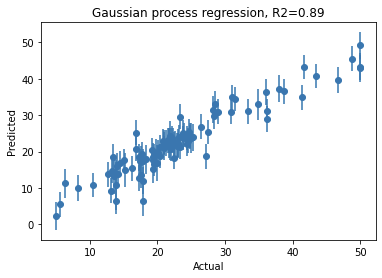
Note that you can get similar performance with other machine learning models such as random forest regressor, etc. However, the key benefit from GPR is that for each given test data point, the predicted value naturally comes with confidence intervals. So not only do you know your model performance, but you know what is the uncertainty associated with each prediction.

This is a high-level overview of GP and GPR. We won’t go into details of the kernels here. But by adopting different kernels, you can incorporate your prior assumptions about the data into your model. With the simple example with scikit-learn, we hope to provide some inspirations in seeing how GPR is useful and you can quickly get started to incorporate some form of Bayesian modeling as part of your machine learning toolbox!

Additional resources

https://distill.pub/2019/visual-exploration-gaussian-processes/ https://nbviewer.jupyter.org/github/adamian/adamian.github.io/blob/master/talks/Brown2016.ipynb