Bayesian inference using Markov Chain Monte Carlo with Python (from scratch and with PyMC3)

9 minute read

A guide to Bayesian inference using Markov Chain Monte Carlo (Metropolis-Hastings algorithm) with python examples, and exploration of different data size/parameters on posterior estimation.

MCMC Basics

Monte Carlo methods provide a numerical approach for solving complicated functions. Instead of solving them analytically, we sample from distributions in approximating the solutions. I have recently written an article on Monte Carlo integration — for which we can use sampling approaches in solving integration problems.

However, there are times when direct sampling from a distribution is not possible. Suppose we wish to sample from \(P(x)\),

\[P(x) = \frac{f(x)}{K}\]

Here we know \(f(x)\), but \(K\) can be difficult to estimate. As a result, we do not know what \(P(x)\) looks like. We cannot directly sample from something we do not know.

Markov chain Monte Carlo (MCMC) is a class of algorithms that addresses this by allowing us to estimate \(P(x)\) even if we do not know the distribution, by using a function \(f(x)\) that is proportional to the target distribution \(P(x)\).

How MCMC solves this is by constructing a Markov chain of \(x\) values such that the stationary distribution of the chain \(\pi(x)\) is equal to \(P(x)\). With some derivation, we can show the following general steps,

Steps

Initialize to some values of \(x\)
For \(t\) = 1, 2, 3, … \(N\)

a. Propose new \(x\) based on a proposal distribution \(q\)

b. Calculate the acceptance ratio \(r\) and acceptance probability \(A\)
\[r(x^*, x^{(t)}) = \frac{f(x^*)q(x^{(t)}|x^*)}{f(x^{(t)})q(x^*|x^{(t)})}\] \[A = \min(1, r(x^*, x^{(t)}))\]
c. Accept the new \(x\) according to acceptance probability A

Different MCMC algorithms define different proposal distributions (aka transition operators). From this you can see that the term Monte Carlo in MCMC refers to the random generation of \(x\) proposals and Markov chain refers to the chain of \(x\)’s formed over the iterations. After an initial burn-in period (where the \(x\) is not stable), the distribution of \(x\) resembles \(P(x)\).

MCMC for Bayesian inference

MCMC is particularly useful in Bayesian inference where we would like to know the posterior estimate of our model parameters — i.e. what is the confidence range of the parameters \(\theta\), given observed data \(X\).

By Bayes’ theorem,

\[p(\theta|x) = \frac{p(x|\theta)p(\theta)}{p(x)} = \frac{p(x|\theta)p(\theta)}{\int p(x|\theta)p(\theta) \,d\theta}\] \[\begin{align*} &p(x|\theta) \text{ is the likelihood} \\ &p(\theta) \text{ is the prior} \\ &p(\theta|x) \text{ is the posterior} \\ &p(x) \text{ is the evidence} \\ \end{align*}\]

A brief note on notation: in some places, you will see the following notation being used,

\[\pi(\theta|x) = \frac{L(\theta)\pi(\theta)}{\int L(\theta)\pi(\theta) \,d\theta}\]

For the remainder of this article, I will continue to use the \(p\) notation.

What the Bayes’ theorem says is that in order to calculate the posterior \(p(\theta|X)\), we need to calculate the product of the likelihood \(p(X|\theta)\) and the prior \(p(\theta)\) over a normalizing factor (the evidence). But the integral term for the normalizing factor is often complicated and unknown. But notice that the posterior is proportional to the product of the likelihood and prior,

\[p(\theta|x) \propto p(x|\theta)p(\theta)\]

This is exactly similar to the expression \(P(x)=f(x)/K\) discussed in the earlier section. Thus, the steps to apply MCMC is exactly the same — we will change the notations to that in the context of Bayesian inference,

Steps

Initialize to some values of \(\theta\)
For \(t\) = 1, 2, 3, … \(N\)

a. Propose new \(\theta\) based on a proposal distribution \(q\)

b. Calculate the acceptance ratio \(r\) and acceptance probability \(A\)
\[r(\theta^*, \theta^{(t)}) = \frac{f(\theta^*|x)q(\theta^{(t)}|\theta^*)}{f(\theta^{(t)}|x)q(\theta^*|\theta^{(t)})}\] \[A = \min(1, r(\theta^*, \theta^{(t)}))\]
c. Accept the new \(\theta\) according to acceptance probability A

Here we are defining \(f\) as the unnormalized posterior, where,

\[f(\theta|x) = p(x|\theta)p(\theta)\]

Note that MCMC is not an optimization algorithm where we try to find the parameter values that e.g. maximize the likelihood. Instead, the result of MCMC is the stationary distribution — it gives us probabilities on the parameters. From this posterior distribution, we know the mean and variance of our estimate on the model parameters given the observed data.

Convergence

How do we know if the MCMC has converged? There are several approaches. The most straightforward way is in examining the trace (i.e. a plot of \(\theta\) over iterations). The trace of the burn-in would look quite different from the trace after convergence. Example,

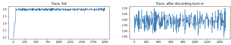
Comparison of trace with and without burn-in. There is an initial period (the burn-in) where the proposals of θ is not yet stable.

As the newly proposed \(\theta\) is dependent on the current \(\theta\), we expect some autocorrelation in the Markov chain — the samples are not completely independent. It can be shown that the error of the estimation in MCMC is,

\[\sigma^2 \approx \frac{\tau}{N} \text{Var}_{p(\theta|x)}[ \theta|x ]\]

where 𝜏 is the integrated autocorrelation time of the chain and represents the steps needed before it is no longer dependent. In fact this is not so different from the variance of a sampling distribution \(\sigma^2/N\), except now we are using an effective sample size (\(N/\tau\)) to account for the autocorrelation. Thus, to minimize error, either we need to reduce the autocorrelation and/or increase the number of samples. It is briefly worth mentioning that an approach to reduce autocorrelation is via thinning — by taking the every \(n\)th sample after convergence for constructing the distribution.

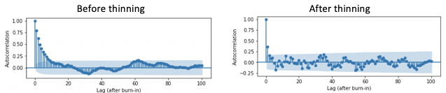
Effects of thinning. Autocorrelation of trace is shown (with burn-in discarded).

However, based on several analyses, it is recommended to increase the sample size \(N\). Thinning, albeit removes autocorrelation, comes with the trade-off of also removing samples that would have otherwise also reduced variance.

There are more statistically rigorous ways to assess convergence that we will not go into more detail in this article: Geweke (1992), Gelman and Rubin (1992), Raftery and Lewis (1992), Heidelberger-Welch (1981; 1983).

Implementation considerations

If we are going to implement the above steps, there is another consideration we need to mention. With many data samples, the likelihood term \(p(X|\theta)\) is the product of all the \(p(X_i|\theta)\) likelihoods (of each sample). Multiplying many probabilities for simulation will lead to very small numbers. Instead, for numerical stability during computational simulation, we need to use the log transform instead. This means we are calculating the log of unnormalized posterior,

\[\ln{p(\theta|x)} \propto \ln{p(x|\theta)p(\theta)}\]

Correspondingly, the acceptance ratio is,

\[\begin{align*} r(\theta^*, \theta^{(t)}) &= \exp\left(\frac{\ln{f(\theta^*|x)}}{\ln{f(\theta^{(t)}|x)}}\right) \frac{q(\theta^{(t)}|\theta^*)}{q(\theta^*|\theta^{(t)})} \\ &= \exp(\ln{f(\theta^*|x)} - \ln{f(\theta^{(t)}|x)}) \frac{q(\theta^{(t)}|\theta^*)}{q(\theta^*|\theta^{(t)})} \end{align*}\]

Metropolis-Hastings in python

The steps presented above is effectively the Metropolis-Hastings (MH) algorithm. The Metropolis algorithm (with symmetric proposal distribution) and Gibbs sampling (sample from conditional distribution, consequently with acceptance ratio equaling 1) are special cases of the MH algorithm.

First we can generate a synthetic observed data \(X\) from a Gaussian distribution, \(X{\sim}\mathcal{N}(3,1)\).

import numpy as np
import scipy.stats as st

# generate observed data
X = st.norm(loc=3, scale=1).rvs(size=1000)

For this example, our likelihood is a Gaussian distribution, and we will use a Gaussian prior \(\theta{\sim}\mathcal{N}(0,1)\). Since Gaussian is a self-conjugate, the posterior is also a Gaussian distribution.

We will set our proposal distribution as a Gaussian distribution centered as the current proposed \(\theta\). The standard deviation of this proposal distribution describes then how far the new \(\theta^*\) proposal is likely to be from the current proposed \(\theta\).

Since the proposal distribution is symmetric, the MH algorithm below technically reduces to the Metropolis algorithm. The \(q(\theta^{(t)}/\theta^*)/q(\theta^*/\theta^{(t)})\) ratio is still included in the code below for didactic purposes,

def guassian_posterior(X, theta):
    # returns the unnormalized log posterior
    loglik = np.sum(np.log(st.norm(loc=theta, scale=1).pdf(X)))
    logprior = np.log(st.norm(loc=0, scale=1).pdf(theta))
    
    return loglik + logprior
    
def guassian_proposal(theta_curr):
    # proposal based on Gaussian
    theta_new = st.norm(loc=theta_curr, scale=0.2).rvs()
    return theta_new

def guassian_proposal_prob(x1, x2):
    # calculate proposal probability q(x2|x1), based on Gaussian
    q = st.norm(loc=x1, scale=1).pdf(x2)
    return q

def mcmc_mh_posterior(X, theta_init, func, proposal_func, proposal_func_prob, n_iter=1000):
    # Metropolis-Hastings to estimate posterior
    thetas = []
    theta_curr = theta_init
    accept_rates = []
    accept_cum = 0
    
    for i in range(1, n_iter+1):
        theta_new = proposal_func(theta_curr)
        
        prob_curr = func(X, theta_curr)
        prob_new = func(X, theta_new)
        
        # we calculate the prob=exp(x) only when prob<1 so the exp(x) will not overflow for large x
        if prob_new > prob_curr:
            acceptance_ratio = 1
        else:
            qr = proposal_func_prob(theta_curr, theta_new)/proposal_func_prob(theta_curr, theta_new)
            acceptance_ratio = np.exp(prob_new - prob_curr) * qr
        acceptance_prob = min(1, acceptance_ratio)
        
        if acceptance_prob > st.uniform(0,1).rvs():
            theta_curr = theta_new
            accept_cum = accept_cum+1
            thetas.append(theta_new)
        else:
            thetas.append(theta_curr)
            
        accept_rates.append(accept_cum/i)
        
    return thetas, accept_rates

# run MCMC
thetas, accept_rates = mcmc_mh_posterior(X, 1, 
                                         guassian_posterior, guassian_proposal, guassian_proposal_prob, 
                                         n_iter=8000)

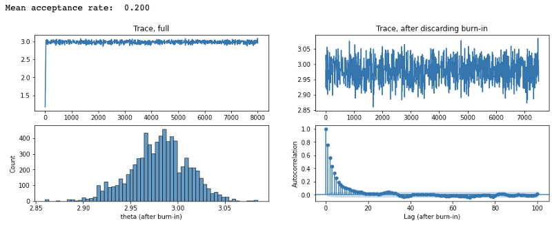
The results look like

from statsmodels.graphics.tsaplots import plot_acf
import matplotlib.pyplot as plt
import seaborn as sns

def plot_res(xs, burn_in, x_name):
    # plot trace (based on xs), distribution, and autocorrelation

    xs_kept = xs[burn_in:]
    
    # plot trace full
    fig, ax = plt.subplots(2,2, figsize=(15,5))
    ax[0,0].plot(xs)
    ax[0,0].set_title('Trace, full')
    
    # plot trace, after burn-in
    ax[0,1].plot(xs_kept)
    ax[0,1].set_title('Trace, after discarding burn-in')

    # plot distribution, after burn-in
    sns.histplot(xs_kept, ax=ax[1,0])
    ax[1,0].set_xlabel(f'{x_name} (after burn-in)')
    
    # plot autocorrelation, after burn-in
    plot_acf(np.array(xs_kept), lags=100, ax=ax[1,1], title='')
    ax[1,1].set_xlabel('Lag (after burn-in)')
    ax[1,1].set_ylabel('Autocorrelation')

plot_res(thetas, 500, 'theta')
print(f"Mean acceptance rate: {np.mean(accept_rates[500:]): .3f}")

While coding this from scratch is a great didactic exercise, we can actually use PyMC3 to do most of the work for us,

import pymc3 as pm

with pm.Model() as model:

    prior = pm.Normal('mu', mu=0, sigma=1)  # prior
    obs = pm.Normal('obs', mu=prior, sigma=1, observed=X)  # likelihood
    step = pm.Metropolis()

    # sample with 3 independent Markov chains
    trace = pm.sample(draws=50000, chains=3, step=step, return_inferencedata=True)  

pm.traceplot(trace)
pm.plot_posterior(trace)

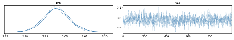
The outputs from PyMC3 looks like,

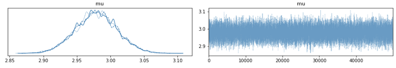
Posterior estimation using PyMC3 with MH algorithm. 50000 iterations.

Note we defined to use Metropolis-Hastings. But there are much more efficient algorithms (e.g. NUTS) also implemented in PyMC3, and can be easily switched for use.

Posterior estimation using PyMC3 with NUTS algorithm. 1000 iterations.

Effects on posterior estimations

Before we conclude, we will run our code on several different scenarios to gain more insights into MCMC. First, we can vary the sample size of the observed data,

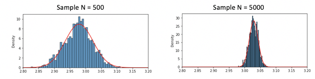
Effects of observed data sample size on variance of posterior estimation. Analytical solution for the posterior per given sample size is shown in red.

We see that with smaller observed dataset, we expectedly see the larger variance in our posterior estimation.

Next, we can vary the standard deviation used in the proposal distribution to observe good versus bad MCMC runs,

MCMC results with SD for proposal distribution = 0.2

MCMC results with SD for proposal distribution = 5

MCMC results with SD for proposal distribution = 0.0001

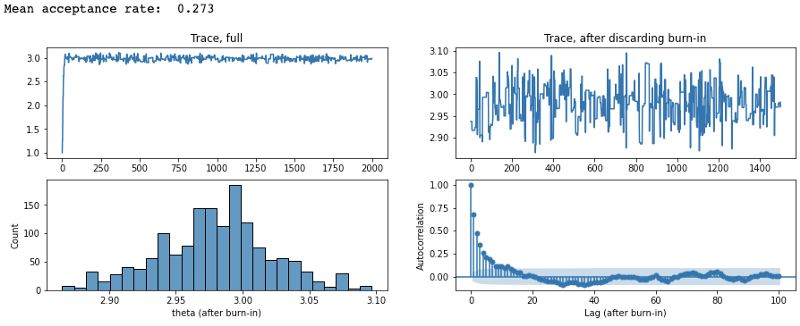
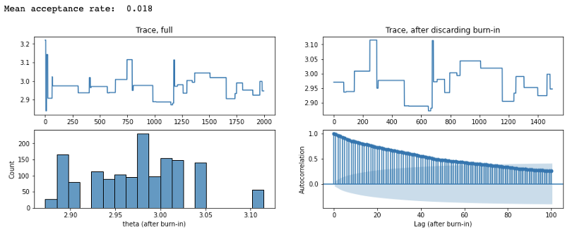
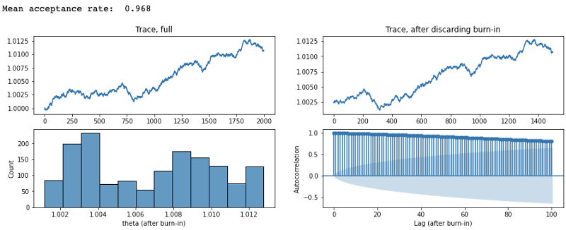
From these, we can see that when the proposal step size is too large, the proposed \(\theta\) is very far from the mean of the target distribution and keep getting rejected (acceptance rate was 1.8%). This results in the trace barely moving to new \(\theta\)’s. Conversely, when we make our proposal step size too small, our acceptance rate is very high (97%) and it takes a long time before the chain ‘forgets’ the previous proposals (as supported by the high autocorrelation). Thus, an optimal acceptance rate (in the case of Gaussian posteriors, ~0.23) is important in having the MCMC reach convergence and in the resulting stationary distribution to be reflective of the target distribution.

Additional resources

Lecture notes

Goodman (2005) Lecture notes on Monte Carlo Methods
Dietze (2012) Lectures 11 (MCMC) and 12 (Metropolis)
Haugh (2017) MCMC and Bayesian Modeling
Breheny (2013) MCMC Methods: Gibbs and Metropolis

Article posts

PyMC3

Share on

Twitter Facebook LinkedIn

Boyang Zhao