Basics of few-shot learning with optimization-based meta-learning

7 minute read

Many machine learning models (particularly deep neural nets) require extensive training data. The idea of few-shot learning is to find ways to build models that can accurately make predictions given just a few training examples. For instance, given models trained on identifying dolphins, traditionally to have a model that can identify dogs possibly means starting from scratch by collecting thousands of dog images and create a new model for this task. With few-shot learning, the goal is to first build models that learn on how to learn quickly given a few images of a new animal (perhaps by learning more generically on what makes one animal different from another) - such that given just one image of a dog, the model can identify dogs in all unseen images. Learning to learn is the premise behind meta-learning.

Meta-learning approaches can be broadly classified into metric-based, optimization-based, and model-based approaches. In this post, we will mostly be focusing on the mathematics behind optimization-based meta-learning approaches.

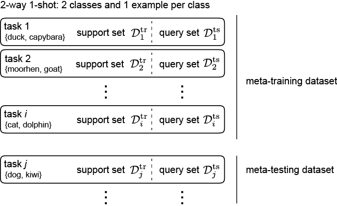
Terminologies. Meta-learning models are trained with a meta-training dataset (with a set of tasks $\tau = \{\tau_1, \tau_2, \tau_3, …\}$) and tested with a meta-testing dataset (tasks $\tau_{\text{ts}}$). Each task $\tau_i$ consists of task training set (i.e. support set) $\mathcal{D}_i^{\text{tr}}$ and task test set (i.e. query set) $\mathcal{D}_i^{\text{ts}}$. One type of meta-learning problems is N-way k-shot learning, in which we choose between N classes and learn with k examples per class.

An example overview of datasets in meta-learning, with 2-way 1-shot learning. The goal is to have a model that can classify amongst two types of animals given just one image of each animal. Here with each task, a support set consists of two labeled images (of two animals, one image each), and query set consists of a set of images for these two animals. Each task contains a different set of two animals. A set of tasks constitute a meta-training dataset used to train the model, and another reserved as meta-testing dataset for validating the model.

Transfer learning (fine-tuning)

Before going on to discuss meta-learning, we will briefly mention another commonly used approach - transfer learning via fine-tuning, to transfer knowledge from a base model (e.g. built by identifying many different objects) to a novel task (e.g. identifying specifically dogs). Here the idea is to build models pre-trained on general tasks, and fine-tune the model on a new specific task (either by only updating limited set of layers in a neural network and/or with a slower learning rate). We will go over the mathematical terminologies in this section, so we can compare and contrast with meta-learning to be discussed later.

In a fine-tuning setting, we would first derive an optimized set of parameters $\theta_{\text{pre-tr}}$ pre-trained on $\mathcal{D}^{\text{pre-tr}}$,

\[\theta_{\text{pre-tr}} = \theta_0 - \alpha \nabla_{\theta} \mathcal{L}(\theta, \mathcal{D}^{\text{pre-tr}})\]

During fine-tuning, we would then tune the parameters that minimize the loss to training set $\mathcal{D}^{\text{tr}}$,

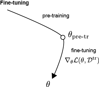
\[\theta = \theta_{\text{pre-tr}} - \alpha \nabla_{\theta} \mathcal{L}(\theta, \mathcal{D}^{\text{tr}})\]

The equation illustrates one gradient step, but in practice this is optimized via multiple gradient steps. As an illustration, below shows the paths in the parameter space going from the pre-trained parameter values $\theta_{\text{pre-tr}} $ toward the fine-tuned parameter values $\theta$.

Meta-learning

In transfer learning via fine-tuning, the hope is that the base model have learned the basic patterns (such as shapes, contrasts, objects in images) that fine-tuning can more quickly and easily adopt to a new task. However, the approach is not specifically designed explicitly around learning to learn. The novel task may not overlap with the base tasks and result in poor performance for the transfer of knowledge. Meta-learning, on the other hand, is designed explicitly around constructing tasks and algorithms for generalizable learning.

MAML

Model agnostic meta-learning (MAML) was proposed by Finn et al in 2017¹. This is an optimization-based meta-learning approach. The idea is that instead of finding parameters that are good for a given training dataset or on a fine-tuned training set, we want to find optimal parameters that with fine-tuning are generalizable to other test sets.

For one task. Given a task, we will first use a support training dataset $\mathcal{D}^{\text{tr}}$ in a fine-tuning step. The optimal parameter $\phi$ for $\mathcal{D}^{\text{tr}}$ is,

\[\phi = \theta - \alpha \nabla_{\theta} \mathcal{L}(\theta, \mathcal{D}^{\text{tr}})\]

Unlike fine-tuning (which we would have stopped here), we want to calculate how well this optimal parameter $\phi$ do on a query test dataset $\mathcal{D}^{\text{ts}}$, with the loss function as $\mathcal{L}(\phi, \mathcal{D}^{\text{ts}})$. The objective is optimize the initial parameter $\theta$ such that it would perform well on the query test set given fine-tuning. In other words, we update $\theta$ in a meta-training step as,

\[\theta = \theta - \beta \nabla_{\theta} \mathcal{L}(\phi, \mathcal{D}^{\text{ts}})\]

Here we need to calculate $\nabla_{\theta} \mathcal{L}(\phi, \mathcal{D}^{\text{ts}})$, which is the derivative of the loss function with respect to $\theta$.

We can illustrate the paths in the parameter space as follows,

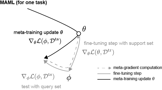
Note that instead of directly updating $\theta$ at the finetuning step, we get a sense on the direction toward the optimal parameters based on the support train and test datasets (paths in gray), and update $\theta$ in the meta-training step.

For task sets. Instead of just one task, for generalizability across a variety of tasks, we can perform this meta-learning at each step by averaging across a set of tasks $\tau = \{\tau_1, \tau_2, \tau_3, …\}$. Hence the optimal parameter $\phi_i$ for task $\tau_i$ of support set is,

\[\phi_i = \theta - \alpha \nabla_{\theta} \mathcal{L}(\theta, \mathcal{D}_i^{\text{tr}})\]

The meta-training step is,

\[\theta = \theta - \beta \nabla_{\theta} \sum_{i} \mathcal{L}(\phi_i, \mathcal{D}_i^{\text{ts}})\]

The term $\nabla_{\theta} \mathcal{L}(\phi_i, \mathcal{D}_i^{\text{ts}})$ can be further expanded. Below we will omit the subscript $i$, but the discussion is applicable as on a per-task basis. With chain rule the term can be expressed as,

\[\begin{align*} \nabla_{\theta} \mathcal{L}(\phi, \mathcal{D}^{\text{ts}}) &= \nabla_{\phi} \mathcal{L}(\phi, \mathcal{D}^{\text{ts}}) \nabla_{\theta} \phi \\ &= \nabla_{\phi} \mathcal{L}(\phi, \mathcal{D}^{\text{ts}}) \nabla_{\theta} \left( \theta - \alpha \nabla_{\theta} \mathcal{L}(\theta, \mathcal{D}^{\text{tr}}) \right) \\ &= \nabla_{\phi} \mathcal{L}(\phi, \mathcal{D}^{\text{ts}}) \left( I - \alpha \nabla^2_{\theta} \mathcal{L}(\theta, \mathcal{D}^{\text{tr}}) \right) \\ \end{align*}\]

We can expand on the earlier path visuals to include multiple tasks,

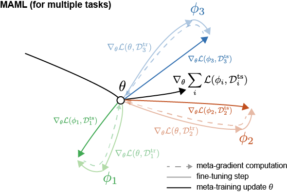
Here we get a sense on the directionality toward the optimal parameters for each task (in different colors), and update $\theta$ based on the average across the tasks (path in black).

First order MAML

In the MAML meta-learning step, we need to calculate the Hessian matrix. As an alternative, in first-order MAML (FOMAML), a first-order approximation can be used by regarding $\nabla_{\theta} \mathcal{L}(\theta, \mathcal{D}^{\text{tr}})$ as a constant and hence ignoring the second derivative terms. This means we treat the term $\nabla_{\theta} \phi$ as identity matrix $I$, resulting in,

\[\nabla_{\theta} \mathcal{L}(\phi, \mathcal{D}^{\text{ts}}) \approx \nabla_{\phi} \mathcal{L}(\phi, \mathcal{D}^{\text{ts}})\]

This can be illustrated visually as follows,

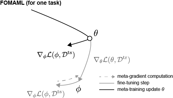
Note we are not performing a meta-gradient computation by unrolling all the way up the computation graph, but instead we are using the first-order approximation $\nabla_{\phi} \mathcal{L}(\phi, \mathcal{D}^{\text{ts}})$ as gradient for updating $\theta$.

Reptile

Reptile (by OpenAI)² is an alternative approach with performance on-par with MAML, but more computationally and memory efficient than MAML as there is no explicit calculations of the second derivatives.

First we’ll introduce an update function $U^k$, which is just a reformulation (and generalization) of the fine-tuning step in MAML,

\[\phi = U_{\tau}^k (\theta, \mathcal{D}^{\text{tr}})\]

where $k$ is the number of times $\phi$ is updated.

With Reptile, at each iteration, 1) a task $\tau_i$ is sampled, 2) the optimal parameter $\phi_i$ for $\tau_i$ is calculated after $k$ updates, and 3) the model parameter $\theta$ is updated as,

\[\theta = \theta + \beta (\phi_i - \theta)\]

Instead of one task per iteration, multiple tasks can be evaluated, leading to a batch version as follows,

\[\theta = \theta + \beta \frac{1}{n} \sum_{n=1}^n (\phi_i - \theta)\]

where $\phi_i = U_{\tau_i}^k (\theta, \mathcal{D}^{\text{tr}})$

The parameters path can be schematically visualized as,

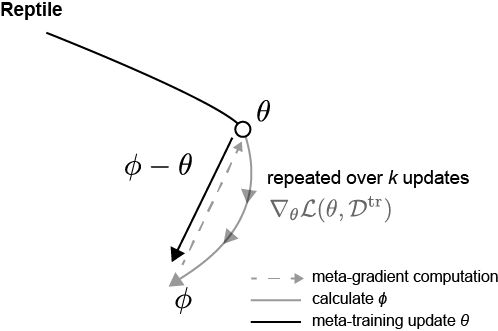
The key distinction that differentiates Reptile from it being just a regular stochastic gradient descent averaged across different tasks is the estimation of $\phi_i$ over $k>1$ steps and using $\phi_i - \theta$ as the gradient for updating $\theta$. In the vanilla stochastic gradient descent, the parameters are updated after each gradient step ($U^1$, where $k=1$). The authors Nichol et al. have showed that when $k>1$, this allows the algorithm to pick up on the higher-order derivatives, and the consequent behavior is similar to MAML and distinctly different from when $k=1$.

Resources

References

Finn et al. Model-Agnostic Meta-Learning for Fast Adaptation of Deep Networks. ICML 2017. arXiv ↩
Nicol et al. On First-Order Meta-Learning Algorithms. arXiv 2018. arXiv ↩

Share on

Twitter Facebook LinkedIn

Boyang Zhao