Understanding binary classifier model structure based on Shapley feature interaction patterns

I have written a full version of this article, available on bioRxiv. A copy of which is presented below.

Introduction

Model explainability is an important part of machine learning and critical in understanding factors that are driving a model’s decision. This includes using models to understand genomic drivers of cellular phenotypes. A myriad of techniques have been developed, including model-agnostic approaches such as SHAP¹, which is based on Shapley values². However, often the emphasis is placed on a ranked list of global feature importance with less attention paid to feature interactions. At best feature interactions are at the level of understanding a feature’s main effect and basic trends of feature interaction. The question remains in how different model structures relate to for example the often used Shapley values, its marginal contributions, and dependence plots.

While several approaches exist for assessing feature interactions such as H-statistics³, partial dependence plot-based variable importance⁴, variable interaction networks⁵, etc, we focus primarily on Shapley/SHAP interactions. This is because of their wide spread usage and they are based on a strong foundations of game theory and are model agnostic. Here, we systemically build binary classifiers with different feature interactions, and observe its impact on Shapley values and contributions.

Feature contribution with Shapley values

Shapley values was developed as an approach in cooperative game theory to estimate the contribution of each player in a coalitional game consisted of multiple players. In the context of machine learning, an individual player corresponds to a feature in a model. Let $\boldsymbol{x} \in \mathbb{R}^M $ be the $M$ features in the model.

The Shapley value for the ith feature is given by \begin{equation} \phi_i = \sum_{S \subseteq F \setminus {i}} \frac{|S|! (|F|-|S|-1)!}{|F|!} (v(S \cup {i}) - v(S)) \end{equation}

where $F$ is the set of all $M$ features and $S$ is a subset of the features ($S \subseteq F$). The function $v(S)$ is a characteristic function that returns the expected payoffs of a given coalition (i.e. model evaluation based on a subset of features). For each given feature subset $S$, we calculate the payoffs of coalitions of $S$ with and without the ith feature. The difference of the two represents the marginal contribution of the ith feature given $S$, of which we weight over all permutations in which the coalition of $S$ can be formed. This is repeated to sum over all feature subsets not containing the ith feature. The resulting Shapley value describes the contribution (or impact) of the ith feature of a given model.

Lundberg and Lee¹ introduced SHAP values by applying Shapley values to machine learning models and defined the characteristic function $v$ as a conditional expectation function,

\[\begin{align} v(S) &= \text{E}[f(\boldsymbol{x}) \vert \boldsymbol{x}_S] \\ \label{eq:v_expect} &= \text{E}_{\boldsymbol{x}_{\bar{S}} \vert \boldsymbol{x}_S}[ f(\boldsymbol{x}_{\bar{S}}, \boldsymbol{x}_{S}) ] = \int f(\boldsymbol{x}_{\bar{S}}, \boldsymbol{x}_S) p(\boldsymbol{x}_{\bar{S}} \vert \boldsymbol{x}_S) \,d \boldsymbol{x}_{\bar{S}} \\ \label{eq:v_expect_ind} &\approx \text{E}_{\boldsymbol{x}_{\bar{S}}}[f(\boldsymbol{x}_{\bar{S}}, \boldsymbol{x}_S)] = \int f(\boldsymbol{x}_{\bar{S}}, \boldsymbol{x}_S) p(\boldsymbol{x}_{\bar{S}}) \,d \boldsymbol{x}_{\bar{S}} \end{align}\]

Here the $v(S)$ is the expectation of the model given coalition of subset features $S$, which is calculated by marginalizing out the other features $\bar{S}$. We simplify Equation \ref{eq:v_expect} to \ref{eq:v_expect_ind} by assuming feature independence⁶. Our discussions below use the approximation Equation \ref{eq:v_expect_ind} when referring to Shapley values. For computational efficiency, several approximation methods (e.g. Kernel SHAP¹, Tree SHAP⁷) have also been introduced for estimating SHAP values.

The Shapley/SHAP values defined thus far relate to the total effect of a single feature. The marginal contribution of the feature in a particular feature set is described in $v(S \cup {i}) - v(S)$. In addition to the total and marginal effects, the effects can also be decomposed into main effects and interaction effects. The SHAP interaction values is based on the Shapley interaction index^8,9, and is defined as⁷, \begin{equation} \label{eq:phi_interact} \phi_{i,j} = \sum_{S \subseteq F \setminus {i,j}} \frac{|S|! (|F|-|S|-2)!}{2(|F|-1)!} \nabla_{ij} (S) \end{equation} where $i \neq j$ and,

\[\begin{align} \nabla_{ij} (S) &= v(S \cup \{i,j\}) - v(S \cup \{i\}) - v(S \cup \{j\}) + v(S) \\ &= [v(S \cup \{i,j\}) - v(S \cup \{j\})] - [v(S \cup \{i\}) - v(S)] \label{eq:phi_interact_v} \end{align}\]

The intuition is that the interaction effect is the difference between the marginal effect of $x_i$ with and without $x_j$. Equation \ref{eq:phi_interact_v} can be rearranged so the marginal effect is of $x_j$. The total interaction is split equally between $\phi_{i,j}$ and $\phi_{i,j}$.

The main effect can be derived as the difference between the total effect $\phi_i$ and the interaction effects $\phi_{i,j}$, \begin{equation} \label{eq:phi_main} \phi_{i,i} = \phi_i - \sum_{i \neq j} \phi_{i,j} \end{equation}

Binary classifier model

We will use a two feature binary classifier model ($\boldsymbol{x} \in \mathbb{R}^2 $), with varying interaction types, to examine their effects.

For $i=1$, there are two feature subsets consisting of $\emptyset$ and ${2}$. The Shapley value for $x_1$ is, \begin{equation} \label{eq:phi_1} \phi_1 = \frac{1}{2} (v({1}) - v(\emptyset)) + \frac{1}{2} (v({1,2}) - v({2})) \end{equation}

For $i=2$, the feature subsets consist of $\emptyset$ and ${1}$, with the Shapley value as, \begin{equation} \label{eq:phi_2} \phi_2 = \frac{1}{2} (v({2}) - v(\emptyset)) + \frac{1}{2} (v({1,2}) - v({1})) \end{equation}

We consider $x \sim U(0,1)$. Given this, the characteristic functions per approximation in Equation \ref{eq:v_expect_ind} are,

\[\begin{align} v(\emptyset) &= \iint f(x_1, x_2) p(x_2) p(x_2) \,dx_1 \,dx_2 \\ v(\{1\}) &= \int f(x_1, x_2) p(x_2) \,dx_2 \\ v(\{2\}) &= \int f(x_1, x_2) p(x_1) \,dx_1 \\ v(\{1,2\}) &= f(x_1, x_2) \end{align}\]

When we examine the characteristic functions of each feature subsets, we can conclude already that $v(\emptyset)$ is a constant; $v({i})$ is related to the main effects of $x_i$ as $x_j$ is integrated out¹⁰, and we will see later this is indeed the case when examining main vs interaction effects; and $v({1,2})$ is just $f(\boldsymbol{x})$. As such, when we decompose $\phi_i$ into the marginal effect components $v({i})-v(\emptyset)$ and $v({1,2})-v({j})$, the first component is the marginal effect of $x_i$ relative to a null feature set and the second component is the marginal effects of $x_i$ relative to a $x_j$ feature set.

We can also directly decompose $\phi_i$ into its main and interaction effects. The interaction effect between $x_1$ and $x_2$ (Equation \ref{eq:phi_interact}) is, \begin{equation} \phi_{1,2} = \frac{1}{2} \left( v({1,2}) - v({1}) - v({2}) + v(\emptyset) \right) \end{equation}

With $\phi_{1,2}$ and $\phi_i$, the main effects (Equation \ref{eq:phi_main}) are,

\[\begin{align} \phi_{1,1} &= v(\{1\}) - v(\{\emptyset\}) \label{eq:phi_11} \\ \phi_{2,2} &= v(\{2\}) - v(\{\emptyset\}) \label{eq:phi_22} \end{align}\]

By this formulation, the main effect of $x_i$ is in fact the same as the marginal component $v({i})-v(\emptyset)$ discussed earlier. Taken together, these mean that changes to the main effects of feature $x_i$ is reflected in $v({i})$ and thus the main effect/marginal effect term $v({i})-v(\emptyset)$; while changes to the feature interactions is reflected in $v({1,2})$ and consequently the interaction effect $\phi_{1,2}$ and the marginal effect term $v({1,2})-v({j})$.

Feature interactions

We can now define $f(\boldsymbol{x})$ with different $x_1$ and $x_2$ interactions. We will first examine logical relations between $x_1$ and $x_2$, starting with an AND relation, and examine how changing this to an OR relation and switching of the inequality signs affect our characteristic functions and resulting dependence plots.

AND operation

Suppose we start with our two-feature model with the following $f(\boldsymbol{x})$,

\[\begin{equation*} f(x_1, x_2) = \begin{cases} 1 & \text{if}\ x_1 > t_1 \text{ and } x_2 > t_2 \\ 0 & \text{otherwise} \end{cases} \end{equation*}\]

The characteristic functions are,

\[\begin{align*} v(\emptyset) &= (1-t_1)(1-t_2) \\ v(\{1\}) &= \begin{cases} 1-t_2 & \text{if}\ x_1 > t_1\\ 0 & \text{otherwise} \end{cases} \\ v(\{2\}) &= \begin{cases} 1-t_1 & \text{if}\ x_2 > t_2\\ 0 & \text{otherwise} \end{cases} \\ v(\{1,2\}) &= \begin{cases} 1 & \text{if}\ x_1 > t_1 \text{ and } x_2 > t_2 \\ 0 & \text{otherwise} \end{cases} \end{align*}\]

The Shapley value for each feature can be decomposed into two components: 1) the marginal contribution of feature to a null-set coalition, 2) the marginal contribution of feature to a coalition consisted of the other feature. For $\phi_1$, this corresponds to $v({1}) - v(\emptyset)$ and $v({1,2}) - v({2})$, respectively.

Combining these two components, as described in Equation \ref{eq:phi_1} and \ref{eq:phi_2}, the Shapley values for the two features are as follows,

\[\begin{align*} \phi_1 &= \begin{cases} \frac{1}{2} t_1 (1-t_2) & \text{if}\ x_1 > t_1 \text{ and } x_2 \leq t_2 \\ (t_1-1)(1-\frac{1}{2} t_2) & \text{if}\ x_1 \leq t_1 \text{ and } x_2 > t_2 \\ t_1 - \frac{1}{2} t_1 t_2 & \text{if}\ x_1 > t_1 \text{ and } x_2 > t_2 \\ \frac{1}{2} (t_1-1)(1-t_2) & \text{otherwise} \\ \end{cases} \\ \phi_2 &= \begin{cases} (t_2-1)(1-\frac{1}{2} t_1) & \text{if}\ x_1 > t_1 \text{ and } x_2 \leq t_2 \\ \frac{1}{2} t_2 (1-t_1) & \text{if}\ x_1 \leq t_1 \text{ and } x_2 > t_2 \\ t_2 - \frac{1}{2} t_1 t_2 & \text{if}\ x_1 > t_1 \text{ and } x_2 > t_2 \\ \frac{1}{2} (t_1-1)(1-t_2) & \text{otherwise} \\ \end{cases} \end{align*}\]

As an example below, we will use, without loss of generality, $t_1=0.8$ and $t_2=0.4$. This corresponds to an upper right region in the feature space where $f(\boldsymbol{x})$ is equal to 1 (Figure 1B). The characteristic function of individual feature subsets concur with our discussions in Section Binary classifier model, viz. $v(\emptyset)$ is a constant, $v({i})$ corresponds to the individual effects of $x_i$, and $v({1,2})$ is $f(\boldsymbol{x})$ (Figure 1C).

Figure 1. Summary of Shapley values for two-feature binary classifier with AND feature relation. (A) Classifier $f(\boldsymbol{x})$ takes the value 1 when both $x_1$ and $x_2$ are above their thresholds. $x \sim U(0,1)$. (B) Heatmap of $f(\boldsymbol{x})$ where dark red region indicates $f(\boldsymbol{x})=1$. (C) Heatmap of each characteristic functions. (D-F) Decomposition of Shapley values into the marginal contributions $v({1}) - v(\emptyset)$ and $v({1,2}) - v({2})$, for $x_1$ (D) and $x_2$ (E), and interaction effects (F). (G) Shapley values for $x_1$ and $x_2$ as dependence plots and heatmaps.

When we examine the decomposition of $\phi_1$, we expectedly observe that the marginal effect $v({1}) - v(\emptyset)$ describes the main effects of $x_1$. The marginal effect $v({1,2}) - v({2})$ describes the additional contribution after having the feature $x_2$ be already added to the coalition. With an ADD relation, this means if $x_2 \leq t_2$, there is no value of $x_1$ that will change $f(x)$ to equal 1 as AND requires also $x_2 > t_2$; consequently the marginal contribution of $x_1$ is zero. On the other hand, when $x_2 > t_2$, values of $x_1$ above threshold $t_1$ exhibits a positive marginal effect, while below threshold a negative marginal effect (Figure 1D). The same behavior is observed for $x_2$ (Figure 1E).

Taken together, we can easily see both the main effects of $x_i$ and the marginal effects of $x_i$ given $x_j$ reflected in the Shapley values $\phi_i$ (Figure 1G). With an ADD feature interaction, when $x_j>t_j$ (this is ‘in-region’ where other feature matters in an ADD relation), $x_i$ will appear to magnify the resulting Shapley values in dependence plots for $\phi_i$ as compared to $x_j \leq t_j$. Furthermore, when both features are above or below their thresholds, they have positive Shapley interaction values; and when one is above and the other is below, they have negative interaction values (Figure 1F).

OR operation

Now let us see what is the effect of changing AND to an OR relation. Here $f(\boldsymbol{x})$ can be defined as,

\[\begin{equation*} f(x_1, x_2) = \begin{cases} 1 & \text{if}\ x_1 > t_1 \text{ or } x_2 > t_2 \\ 0 & \text{otherwise} \end{cases} \end{equation*}\]

The characteristic functions are,

\[\begin{align*} v(\emptyset) &= 1 - t_1 t_2 \\ v(\{1\}) &= \begin{cases} 1 & \text{if}\ x_1 > t_1\\ 1-t_2 & \text{otherwise} \end{cases} \\ v(\{2\}) &= \begin{cases} 1 & \text{if}\ x_2 > t_2\\ 1-t_1 & \text{otherwise} \end{cases} \\ v(\{1,2\}) &= \begin{cases} 1 & \text{if}\ x_1 > t_1 \text{ or } x_2 > t_2 \\ 0 & \text{otherwise} \end{cases} \end{align*}\]

With this, we can derive our Shapley values,

\[\begin{align*} \phi_1 &= \begin{cases} \frac{1}{2} t_1 (t_2+1) & \text{if}\ x_1 > t_1 \text{ and } x_2 \leq t_2 \\ \frac{1}{2} t_2 (t_1-1) & \text{if}\ x_1 \leq t_1 \text{ and } x_2 > t_2 \\ \frac{1}{2} t_1 t_2 & \text{if}\ x_1 > t_1 \text{ and } x_2 > t_2 \\ \frac{1}{2} (t_1-1)(t_2+1) & \text{otherwise} \\ \end{cases} \\ \phi_2 &= \begin{cases} \frac{1}{2} t_1 (t_2-1) & \text{if}\ x_1 > t_1 \text{ and } x_2 \leq t_2 \\ \frac{1}{2} t_2 (t_1+1) & \text{if}\ x_1 \leq t_1 \text{ and } x_2 > t_2 \\ \frac{1}{2} t_1 t_2 & \text{if}\ x_1 > t_1 \text{ and } x_2 > t_2 \\ \frac{1}{2} (t_1+1)(t_2-1) & \text{otherwise} \\ \end{cases} \end{align*}\]

Per discussions in Section Binary classifier model, we note the main/marginal effect $v({i}) - v(\emptyset)$ is independent of the $x_1$ and $x_2$ interactions, whereas the marginal effect $v({1,2}) - v({i})$ is dependent on the interaction. As a result, we expectedly observe that the main effects of $x_i$ remain unchanged, but the marginal effects of $x_i$ given $x_j$ (and interaction effect) to be switched when we change the feature relations from AND to OR. Unlike in the AND relation, if $x_2 > t_2$, $f(\boldsymbol{x})$ is equal to 1 independent of the values of $x_1$ and therefore the marginal contribution of $x_1$ given $x_2 > t_2$ is zero. Conversely, if $x_2 \leq t_2$, then $f(\boldsymbol{x})$ is fully dependent on $x_1$ (Figure 2).

Figure 2. Summary of Shapley values for two-feature binary classifier with OR feature relation. (A) Classifier $f(\boldsymbol{x})$ takes the value 1 when either $x_1$ or $x_2$ are above their thresholds. $x \sim U(0,1)$. (B) Heatmap of $f(\boldsymbol{x})$ where dark red region indicates $f(\boldsymbol{x})=1$. (C) Heatmap of each characteristic functions. (D-F) Decomposition of Shapley values into the marginal contributions $v({1}) - v(\emptyset)$ and $v({1,2}) - v({2})$, for $x_1$ (D) and $x_2$ (E), and interaction effects (F). (G) Shapley values for $x_1$ and $x_2$ as dependence plots and heatmaps.

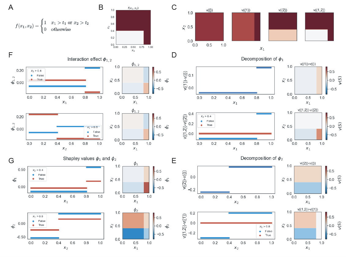
Thus, with an OR relation, when $x_j \leq t_j$, it is ‘in-region’ where $x_i$ matters and $x_i$ will appear to magnify the resulting Shapley values in dependence plots for $\phi_i$, as compared to $x_j > t_j$ (Figure 2G). Furthermore, when both features are above or below their thresholds, they have negative Shapley interaction values; and when one is above and the other is below, they have positive interaction values (Figure 2F).

Inequality sign switch

If the main effects are reflected in the marginal contribution of $v({i}) - v(\emptyset)$, this also means this component is directly affected when we change the direction of inequality. Take for example the function,

\[\begin{equation*} f(x_1, x_2) = \begin{cases} 1 & \text{if}\ x_1 > t_1 \text{ and } x_2 < t_2 \\ 0 & \text{otherwise} \end{cases} \end{equation*}\]

The main effects of $x_i$ can be readily observed in the individual $v({i})$ characteristic functions and the Shapley dependence plots (Figure 3). In fact, we can also easily identify that $x_1$ is associated with a greater than inequality and $x_2$ is associated with a less than inequality based on their respective main effects.

Figure 3. Summary of Shapley values for two-feature binary classifier with AND feature relation; similar to Figure 1, but with inequality direction switched for $x_2$. (A) Classifier where $f(\boldsymbol{x})$ takes the value 1 when both $x_1$ and $x_2$ are above and below their thresholds, respectively. $x \sim U(0,1)$. (B) Heatmap of $f(\boldsymbol{x})$ where dark red region indicates $f(\boldsymbol{x})=1$. (C) Heatmap of each characteristic functions. (D) Shapley values for $x_1$ and $x_2$ as dependence plots and heatmaps.

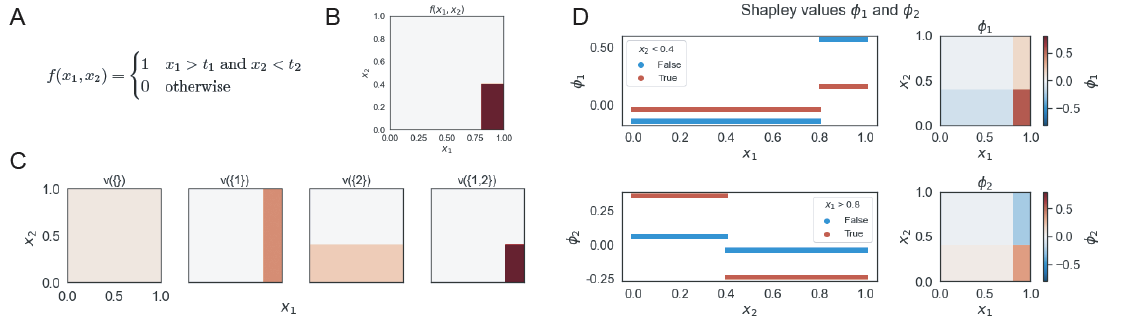
Furthermore, we note from the dependence plots that when $x_1 > t_1$ or $x_2 < t_2$, with an AND relation, they are ‘in-region’ and thus changes to correspondingly $x_2$ or $x_1$ magnifies the Shapley values $\phi_2$ or $\phi_1$, respectively (Figure 3D).

Additivity

Aside from logical operations, we can also construct feature interactions based on arithmetic operations. Suppose we have the following additive feature interaction,

\[\begin{equation*} f(x_1, x_2) = \begin{cases} 1 & \text{if}\ x_1+x_2 > t \\ 0 & \text{otherwise} \end{cases} \end{equation*}\]

The characteristic functions are,

\[\begin{align*} v(\emptyset) &= \begin{cases} \frac{1}{2} (2-t)^2 & \text{if}\ t>1 \\ 1 - \frac{1}{2} t^2& \text{otherwise} \end{cases} \\ v(\{1\}) &= 1 - (t-x_1) \; \text{with } v(\{1\}) \in [0,1] \\ v(\{2\}) &= 1 - (t-x_2) \; \text{with } v(\{2\}) \in [0,1] \\ v(\{1,2\}) &= \begin{cases} 1 & \text{if}\ x_1+x_2 > t \\ 0 & \text{otherwise} \end{cases} \\ \end{align*}\]

In contrast to the logical operations, in the functions with arithmetic operations, the Shapley dependence plots is not a step function (Figure 4) but instead exhibit linear relationships between $\phi_i$ and $x_i$ in defined regions. Our conclusions regarding main vs. interaction effects as discussed in Section Binary classifier model are still applicable. Namely the main effects of $x_i$ are reflected in $v({i}) - v(\emptyset)$. The marginal contribution $v({1,2}) - v({i})$ and interaction effect describes the additive interaction between the two features. The region for which $x_1 + x_2 > t$ results in higher Shapley values. Moreover, in this region, a lower value of $x_j$ results in a higher Shapley value for $\phi_i$ because $x_i$ now needs to contribute more to get past the threshold $t$. There are also some effects of whether $t>1$ or $t<1$, but aside from when the linearity appears, the resulting dependence plots are consistent with the earlier observations.

Figure 4. Summary of Shapley values for two-feature binary classifier with additive feature relation. (A) Classifier where $f(\boldsymbol{x})$ takes the value 1 when the sum $x_1$ and $x_2$ are above threshold $t$. $x \sim U(0,1)$. (B) Heatmap of $f(\boldsymbol{x})$ where dark red region indicates $f(\boldsymbol{x})=1$. (C) Heatmap of each characteristic functions. (D-F) Decomposition of Shapley values into the marginal contributions of $v({1}) - v(\emptyset)$ and $v({1,2}) - v({2})$, for $x_1$ (D) and $x_2$ (E), and interaction effects (F). (G) Shapley values for $x_1$ and $x_2$ as dependence plots and heatmaps.

Several other effects are worth mentioning. As previously discussed in Section Inequality sign switch, switching of the inequality sign correspondingly affects the main effects of each feature. The marginal effects of $x_i$ given $x_j$ and the interaction effects remain additive in nature. In all, the logics in the interrelationships amongst the different contribution components and Shapley values are the same as discussed.

Models with noise

Thus far, we have used noiseless models to gain insights into model structure based on characteristic functions, marginal effects, and Shapley values. These interconnections are retained when we consider models with noise. For this we set a background noise such as $f(\boldsymbol{x}) \sim \text{Bern}(p)$. For approximations, we build a tree ensemble random forest model with feature contributions calculated using SHAP¹¹.

Figure 5. Tree SHAP values for models with noise, Bern(0.2). (A) Binary classifier with AND feature interaction. (B) Binary classifier with additive feature interaction.

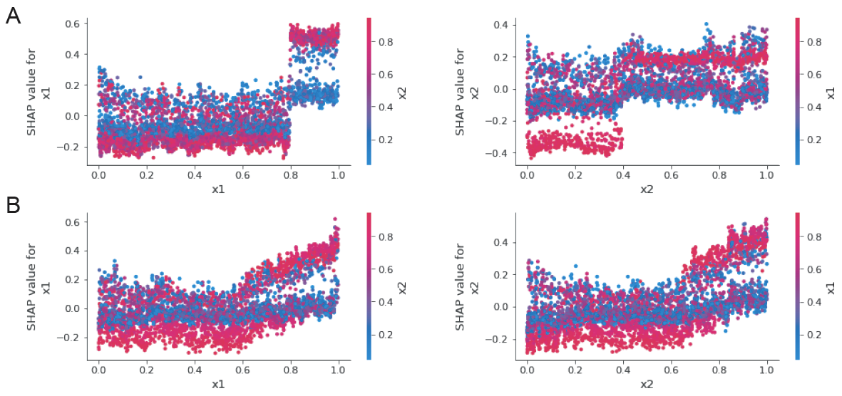
We can distinctly observe that the underlying model for Figure 5A exhibits a logical AND feature interaction whereas that for Figure 5B exhibits additive interaction. The spreads of SHAP values in the dependence are consistent with our earlier discussions of these models.

Conclusion

Model agnostic approaches, such as Shapley values or SHAP, have improved our understanding of black-box models. Here we explored using simple two-feature binary classifiers on how the importance of a feature can be decomposed into its main and interaction effects as well as its marginal contributions. The collective effect, i.e. Shapley value, for a given feature can be readily examined in dependence plots with the underlying decomposed effects remaining prominent. Furthermore, specific interactions exhibit distinct behaviors, such as logical interactions with step-function like dependence or linearly additive interactions with linear dependence. ‘In-region’ interactions further magnify the Shapley values. While the models here were restricted to two-feature models, the underlying decomposition, and their effects are translatable to multi-feature models. Together, we see the inter-connectivity between underlying model structure and Shapley values/interaction patterns.

References/Footnotes

1. S. Lundberg and S.-I. Lee, “A unified approach to interpreting model predictions,” in NIPS, 2017. ↩ ↩² ↩³

2. L. S. Shapley, “A value for n-person games,” Contributions to the Theory of Games, vol. 2, pp. 307–317, 1953. ↩

3. J. H. Friedman and B. E. Popescu, “Predictive learning via rule ensembles,” The Annals of Applied Statistics, vol. 2, no. 3, pp. 916–954, 2008. ↩

4. B. M. Greenwell, B. C. Boehmke, and A. J. McCarthy, “A simple and effective model-based variable importance measure,” 2018. ↩

5. G. Hooker, “Discovering additive structure in black box functions,” in Proceedings of the Tenth ACM SIGKDD International Conference on Knowledge Discovery and Data Mining, KDD ’04, (New York, NY, USA), p. 575–580, Association for Computing Machinery, 2004. ↩

6. The feature independence assumption was made in the SHAP value calculations¹. More recently, Aas et al¹² have extended methods for SHAP calculations allowing for feature dependence. ↩

7. S. M. Lundberg, G. G. Erion, and S.-I. Lee, “Consistent individualized feature attribution for tree ensembles,” arXiv preprint arXiv:1802.03888, 2018. ↩ ↩²

8. K. Fujimoto, I. Kojadinovic, and J.-L. Marichal, “Axiomatic characterizations of probabilistic and cardinal-probabilistic interaction indices,” Games and Economic Behavior, vol. 55, pp. 72–99, 2006. ↩

9. M. Grabisch and M. Roubens, “An axiomatic approach to the concept of interaction among players in cooperative games,” Int. Journal of Game Theory, 1999. ↩

10. We use $j$ to refer to the other feature, given feature $i$, in the two-feature model ↩

11. TreeSHAP⁷ was used. This is a computationally efficient algorithm for approximating SHAP values for tree-based models ↩

12. K. Aas, M. Jullum, and A. Løland, “Explaining individual predictions when features are dependent: More accurate approximations to shapley values,” 2020. ↩